Solving Unified Field Theory

The Structure of Spacetime as the Governor of Real Matter and Energy

A Conceptual Framework and Research Program

How to read this document

This is an outline of a conjecture, not a finished theory. Throughout, I have marked each claim by its status. “Established” means it is confirmed physics. “Open problem” means mainstream cosmology genuinely does not know the answer. “Conjecture” means it is my proposal, not yet tested. I have deliberately kept these separate so that the idea can be judged fairly — on the strength of its reasoning, not on any overstatement.

1. The Central Idea

I want to propose a single organizing principle: that the structure of spacetime at a given location governs how much real matter and energy exist there, by governing the conversion between the quantum vacuum and real, persistent particles. In this picture the universe does not require a creation event. Matter and energy are never made from nothing and never destroyed into nothing; they are converted, back and forth, between a latent vacuum state and a real state, and the exchange rate is set by the geometry of spacetime itself.

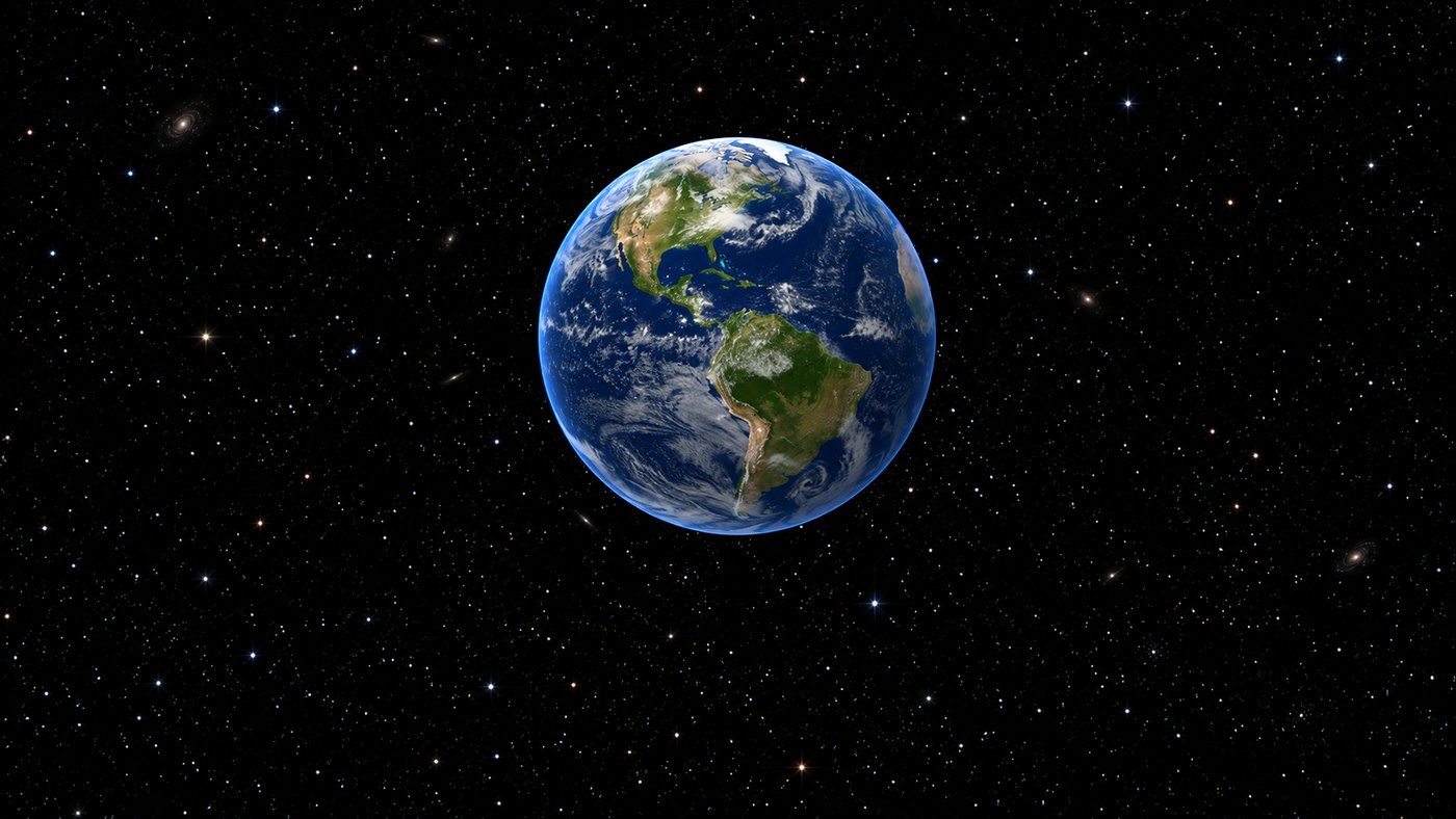
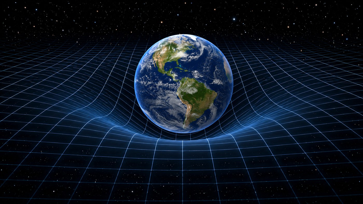
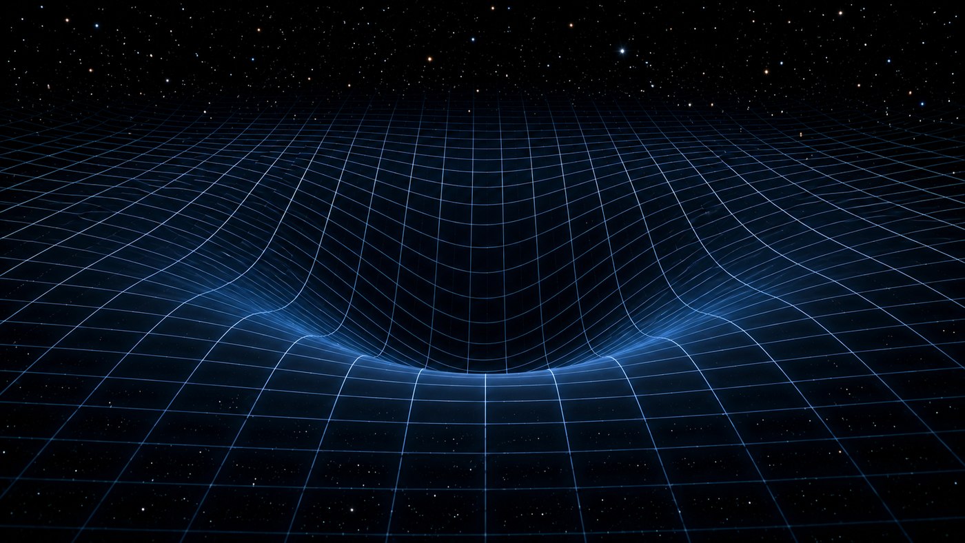
My motivation is a dissatisfaction I take seriously: the standard account traces the universe back to an initial singularity of infinite density. I find that unsatisfying — an infinite-density origin either violates our conservation principles or hides the difficulty behind the phrase “a quantum fluctuation started it.” I think we can do better with a cyclical, conversion-based picture in which nothing is ever created from nothing.

STATUS — Open problem. The initial singularity is openly regarded by cosmologists as the point where general relativity breaks down and a deeper (quantum-gravity) theory is needed. My dissatisfaction is shared; cyclic and bounce cosmologies (Penrose; Steinhardt–Turok; Popławski; loop quantum cosmology) are active research programs built on avoiding this singularity.

2. The Foundation: The Vacuum Is Not Empty

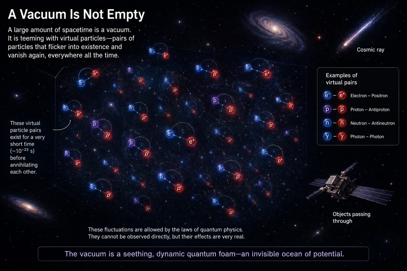
My framework rests on one premise, and I want to establish it firmly because everything else depends on it: empty space is not truly empty. It is a quantum field in its lowest-energy state, perpetually fluctuating, and under the right conditions those fluctuations can be converted into real, measurable particles.

2.1 The Dynamic Casimir Effect

The clearest proof I can point to is the dynamic Casimir effect. If you take a boundary — in practice, a superconducting circuit whose effective length is modulated extremely fast — and change that boundary condition rapidly enough, real photons appear out of the vacuum. This has been demonstrated experimentally. It shows, beyond dispute, that a changing boundary condition converts vacuum fluctuations into real particles. This is the seed of my entire proposal: the vacuum is a reservoir, and the right conditions draw real particles out of it.

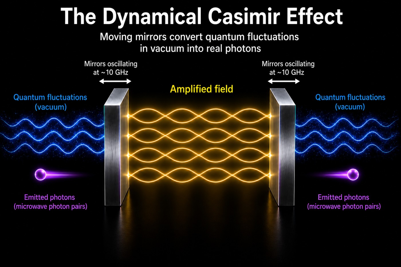
STATUS — Established. The dynamic Casimir effect is confirmed physics, first demonstrated in a superconducting circuit in 2011. The vacuum-to-real-particle conversion it embodies is real.

2.2 From Photons to Matter: The Cost of Mass

The dynamic Casimir effect makes photons, and photons are the cheap case: massless, costing only their quantum of energy, h·f. The conversion my framework cares about must eventually cover matter, and the matter version of the same conversion carries an additional, irreducible price: a particle–antiparticle pair costs at least 2mc² of rest energy before anything else. The laboratory record on that side of the ledger is worth stating precisely, because it brackets what is established and what is frontier.

Routine: pair production near a nucleus. A gamma photon above 1.022 MeV, passing close to a nucleus, converts into an electron–positron pair — observed since 1933 (Blackett and Occhialini) and so thoroughly domesticated that the reverse process is the working principle of PET scanners. Demonstrated, in assisted form: the Breit–Wheeler process, light plus light making matter (Breit and Wheeler, 1934). At SLAC in 1997, experiment E144 collided high-energy photons with an intense laser field and produced electron–positron pairs (Burke et al., 1997) — real, confirmed matter from light. Not yet achieved: the Schwinger effect (Schwinger, 1951) — pulling electron–positron pairs directly out of the vacuum with a strong electric field alone, the closest conceptual cousin of the dynamic Casimir effect on the matter side. It requires field strengths near 10¹⁸ volts per metre, beyond any current laser. It is the frontier, not a done experiment.

This ladder matters for the framework: photon conversion from the vacuum is confirmed (Section 2.1); photon-assisted matter conversion is confirmed; pure vacuum-to-matter conversion is predicted by the same quantum field theory but still untested. My conjecture in Section 3.2 — that location could discount the cost of becoming real — lives at the top of this ladder, in the one regime the laboratory has not yet reached.

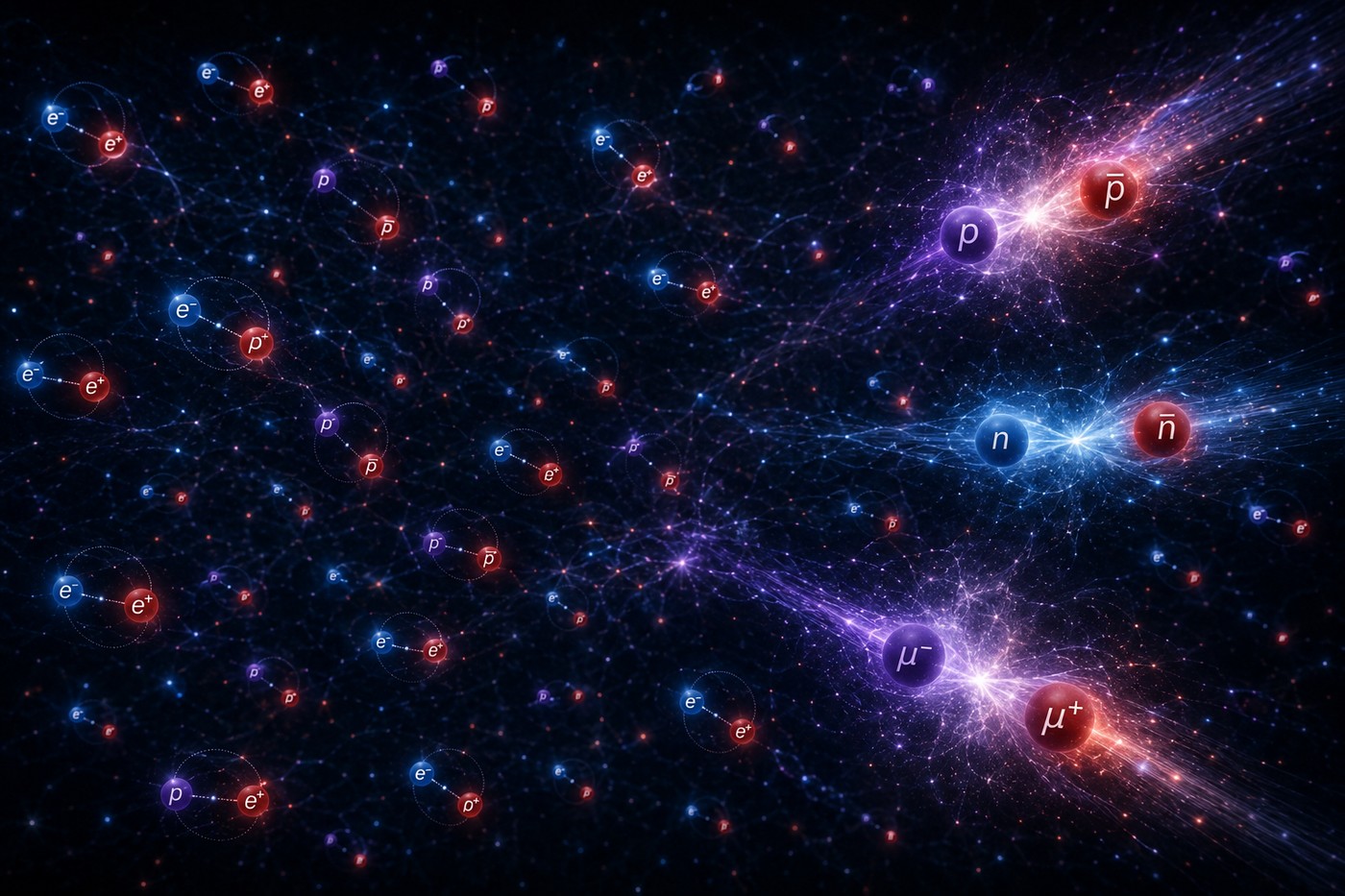
STATUS — Established, except the top rung. Nuclear pair production and the assisted Breit–Wheeler process are confirmed; the pure Schwinger effect is an outstanding prediction of standard quantum field theory, pursued by present-day extreme-light laser facilities. Nothing on this ladder requires my framework — but the framework must be consistent with every rung.

3. Spacetime Curvature Converts the Vacuum into Real Particles

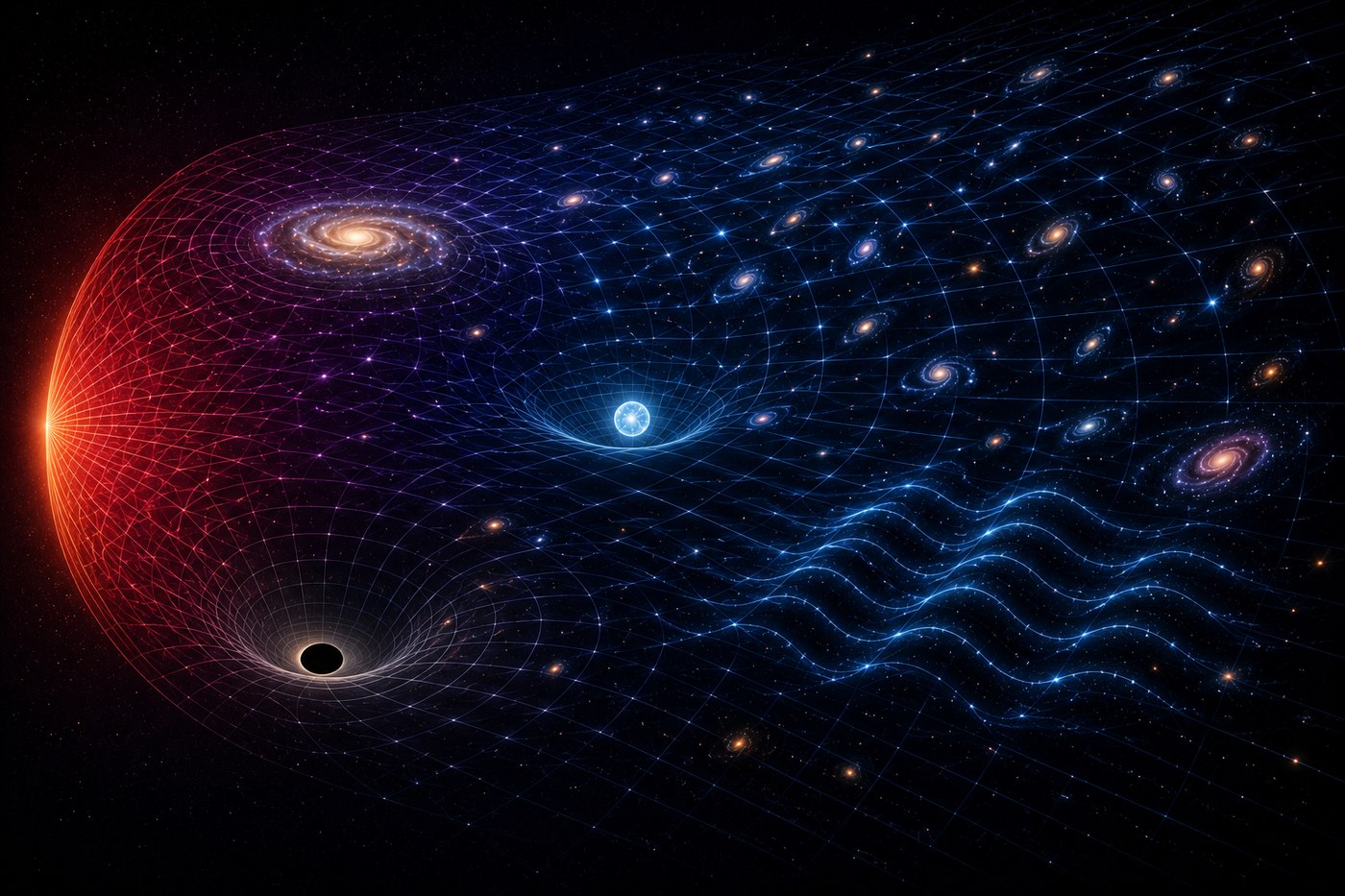
If a fast-changing boundary can draw particles from the vacuum, I propose that the curvature of spacetime does something analogous: it changes the conditions the vacuum must satisfy, and near strongly curved regions the vacuum is “closer” to yielding real particles. I claim that the structure of spacetime is the governing variable that determines where and whether virtual fluctuations become real.

3.1 Gravitational Particle Production and Hawking Radiation

This is not a bare guess — it corresponds to a known effect. In a strongly curved or rapidly changing spacetime, the definition of “empty” shifts, and vacuum fluctuations appear as real particles. This is called gravitational particle production, and its most famous instance is Hawking radiation: near a black hole’s horizon, the geometry can separate a fluctuating pair so that one particle becomes real and escapes. The location — the horizon — is what makes the conversion spontaneous. That is precisely the kind of location-dependence I am proposing as the heart of the framework.

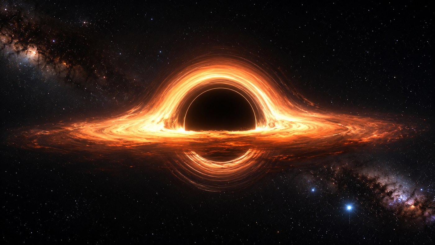
STATUS — Established (with one correction I accept). Gravitational particle production and Hawking radiation are standard theory, and the underlying vacuum-to-particle mechanism is confirmed in laboratory analogs. Current understanding is that the energy of the produced particles comes from the gravitating mass itself, so the process drains its source rather than adding to it. The phenomenon itself — curvature converting vacuum into real particles — is exactly the kind of location-dependence this framework proposes.

STATUS — Conjecture (open regime). It is possible that virtual fluctuations becoming real within or near a black hole, and falling into it, would actually increase the black hole’s mass. Every black hole observed to date has grown, and the evaporation of a black hole has never been observed. I hold this as my conjecture, in a regime the theory cannot yet compute; Section 10.7 records the closest observational test and its current verdict.

I want to be precise about how deep this mechanism runs, because it is not a quirk of one experiment. The dynamic Casimir effect, the Unruh effect, and Hawking radiation are three faces of a single piece of physics. The Unruh effect (Unruh, 1976) says that an observer accelerating through empty vacuum sees it as a warm bath of photons — acceleration alone turns the vacuum into apparent radiation. Hawking radiation is the same idea transplanted to curved spacetime: the event horizon acts as the boundary, and its presence makes the black hole emit particles from the vacuum. And the dynamic Casimir effect of Section 2.1 is the tabletop member of the family: a boundary accelerated fast enough converts vacuum fluctuations into real photons. In all three, the ingredient is identical — a boundary or observer that is accelerated, or a spacetime that changes — and the output is identical: virtual fluctuations promoted to real particles.

The pair structure matters, and it carries the deepest open problem in the subject. A black hole emits particles in entangled pairs: one partner falls in, one escapes. The escaping partner, viewed alone, is exactly thermal — it carries entropy — while the pair together remains a pure quantum state. That mismatch, accumulated over a black hole’s lifetime, is the root of the black-hole information puzzle (Hawking, 1976). The dynamic Casimir effect exhibits precisely the same structure on a tabletop: the converted photons emerge in entangled pairs, each partner alone thermal and entropy-carrying, the pair together pure. For my framework this is important twice over. It confirms that vacuum-to-real conversion is pair-wise and entangling wherever it occurs, in the laboratory and at a horizon alike. And it means any mature version of the conversion term Q (Section 12.2) must track not just energy but entanglement — which is where the entropy bookkeeping of Sections 5 and 10.3 will ultimately have to live.

STATUS — Established mechanism family; open puzzle. The unity of the dynamic Casimir effect, the Unruh effect, and Hawking radiation is standard theory, and the entangled-pair structure of dynamic Casimir photons is measured. What no one knows is how the information comes back out — the puzzle is a live frontier of physics, not a defect of the framework, but any theory claiming to govern the conversion inherits it.

3.2 Redshift: Energy Depends on Location and Epoch

My claim that spacetime structure sets a location-dependent “energy budget” is grounded in relativity itself. A photon climbing out of a gravitational well loses energy as measured by a distant observer (gravitational redshift), and light traveling through expanding space is stretched to lower energy (cosmological redshift). So energy is genuinely location- and epoch-dependent in curved, expanding spacetime. This is the established backbone on which I build.

STATUS — Established. Gravitational redshift is confirmed (Pound–Rebka, 1959; corrected for daily in GPS). Cosmological redshift is the basis of measured cosmic expansion.

A conjecture: I have wondered whether real particles are “cheaper” to create locally near a massive object. The best current physics says the local cost of creating a particle is the same everywhere (the rest energy is a local invariant), and the equivalence principle — the foundation of general relativity — supports this. I therefore hold this only as a conjecture in one regime we cannot yet compute: the interior of a black hole, where the theory itself breaks down and honest physics says “unknown.” Also, the rest energy is really saying how much energy is available at that location due to a real particle. What I am adding is that location-dependent vacuum fluctuations could allow real particles to be pulled from the vacuum with less input than the rest energy.

4. Dark Energy as a Property of Spacetime Structure

If spacetime structure governs the conversion of vacuum to real energy, then the mysterious energy driving cosmic expansion — dark energy — is a natural place for my framework to speak. I propose that dark energy is best understood as a property of spacetime’s structure rather than a substance sitting inside space.

This is not a fringe reframing. In Einstein’s field equations, the cosmological constant enters on the geometry side of the equation — as a feature of spacetime itself, not as ordinary matter or energy. So the interpretation I favor is arguably the original and most conservative one.

STATUS — Open problem. What dark energy is remains unknown. “Cosmological constant” is a placeholder. The naive vacuum-energy calculation disagrees with the observed value by roughly 120 orders of magnitude — often called the worst quantitative mismatch in physics. My framework does not yet resolve this, but it lives squarely on this open question.

4.1 Is Dark Energy Evolving? The Friedmann Test

The expansion history of the universe is governed by the Friedmann equations. When I test my cyclic instinct against them, the result is clarifying and I want to report it honestly. A universe with a fixed cosmological constant expands forever. For the universe to be cyclic — to slow, stop, or reverse — dark energy cannot be a fixed constant; it must evolve over cosmic time.

This is exactly the frontier the data is now probing. The DESI galaxy survey reports a statistically suggestive indication (roughly 2.8 to 4.2 sigma, depending on the supernova dataset used) that dark energy is not constant but evolving. My prediction that “the static-constant picture is incomplete” therefore aligns with the direction of the newest measurements.

Where I am careful: the data currently favors dark energy that evolves but still drives expansion forever; it does not (yet) support an actual reversal into contraction. So the first half of my claim — that dark energy is not a static constant — has genuine observational wind behind it, while the stronger cyclic conclusion remains unconfirmed (the competing trajectories — runaway, recollapse, and closed loop — are drawn explicitly in Figure 2, Section 12.6).

STATUS — Open problem / partially supported. Whether dark energy evolves (whether the parameter wₐ ≠ 0) is unsettled and actively contested right now. This is the single most testable descendant of my framework, and it is a live question, not a closed one.

5. Conservation, Not Creation: Matter, Antimatter, and Entropy

My bedrock commitment is that energy is never created or destroyed, only converted between forms and states. When matter meets antimatter it does not vanish into nothing — it converts to radiation, and that radiation is still with us as the cosmic microwave background. The matter we are made of is the tiny surplus that survived. This is all energy changing form, never disappearing, which is exactly the principle I want to build the cosmos on.

I extend this instinct to the largest scale: I propose that what looks like an expanding, entropy-increasing universe in the “real” sector is balanced by a complementary conversion elsewhere — so that the global books close and no creation event is needed. I offer this as the conjectural heart of the framework.

STATUS — Mixed. Local conservation of energy is established and central to my view — correctly. The subtlety I acknowledge: at cosmic scale, total energy conservation genuinely loosens because expanding spacetime lacks time-translation symmetry. My “balancing sector” is an attempt to restore strict global bookkeeping; as stated it is a conjecture that does not yet make a distinct measurable prediction, and I flag it as such rather than claiming it as fact.

5.1 The Matter–Antimatter Asymmetry

Why the universe kept any matter at all — rather than annihilating completely to light — is unexplained at the deepest level. The leading serious mechanism (leptogenesis, via heavy neutrinos decaying slightly asymmetrically) is unconfirmed. My conversion-based framework is naturally sympathetic to asymmetry-generating processes, though I do not claim to have derived the specific mechanism.

STATUS — Open problem. The origin of the matter–antimatter asymmetry is one of the major unsolved problems in physics. Known physics falls short of explaining the observed surplus.

6. Dark Matter

In earlier drafts I was candid that dark matter was the piece that fit my framework least cleanly, and I claimed nothing. I now think the framework has something to say, and I state it as a flagged conjecture rather than staying silent — with the tests it must pass named in the same breath.

The evidence to be explained is overwhelming and mutually consistent: galaxy rotation curves, gravitational lensing, the CMB peak structure, and the growth of cosmic structure all require roughly five times more gravitating mass than we can see — and no dark matter particle has been detected.

My conjecture: dark matter phenomenology is the gravitating response of the vacuum sector. Pairs of particles flickering in and out of existence carry energy, and energy gravitates; if the conversion between the vacuum and real states depends on the local structure of spacetime (Section 3), then the vacuum’s contribution to gravity is not uniform — it is modulated by the matter that is present, adding effective weight where matter already is. The orbital analysis of Section 7.3 sharpens this with a number. Galaxy rotation curves go anomalous below a specific acceleration, a₀ ≈ 1.2×10⁻¹⁰ m/s² (Milgrom, 1983) — and that acceleration is numerically about cH₀/2π, the acceleration scale of the cosmic horizon itself. The scale at which galactic orbits misbehave is the scale set by cosmic expansion. That published, unexplained coincidence is exactly where a framework coupling local dynamics to the cosmic vacuum ought to live, and it has a serious published counterpart: Verlinde’s emergent gravity (Section 10.2), which derives dark-matter-like effects from the entropy of the vacuum.

Two honest costs, stated plainly. First, raw vacuum energy gravitates as dark energy — smooth, with w = −1 — not as clustering matter; for the vacuum’s weight to clump where the galaxies are, the conversion rate must genuinely depend on local spacetime structure, which is this framework’s central conjecture (Section 3.2), not a result. Second, any picture in which the dark effect is a response to the visible matter inherits the hardest test in the suite: the Bullet Cluster (Section 11, item 5), where the gravitating mass demonstrably separates from the visible gas. Verlinde’s proposal faces the same difficulty, and observational tests of it remain contested. If the framework cannot pass the Bullet Cluster, this section reverts, honestly, to silence.

STATUS — Conjecture (upgraded from silence). The undiscovered-particle explanation remains fully compatible with this framework and may simply be true. My conjecture is an alternative reading: the dark sector as the vacuum’s location-dependent weight, anchored to the a₀ ≈ cH₀/2π coincidence, with Verlinde as its published counterpart and the Bullet Cluster as the test that would send this section back to silence.

7. The Black-Hole Universe and the Avoided Singularity

One current thought for a universe without a creation event is the possibility that our universe is the interior of a black hole formed in a larger parent universe. If a collapsing region, instead of reaching an infinite-density singularity, bounces and expands into a new causally-disconnected region, then that bounce would look, from inside, exactly like a Big Bang. Our expansion would be the expansion of that bounced interior. There would be no creation from nothing — only a conversion from a parent’s collapse into our expansion.

This removes the initial singularity I objected to, replacing an infinite-density origin with a finite bounce that has a “before.”

STATUS — Conjecture with a real counterpart. A black-hole/bounce cosmology (associated with Nikodem Popławski, using torsion in Einstein–Cartan gravity) is a genuine, mathematically-developed, published proposal — though it is a minority view and unconfirmed, because the required high-density torsion physics has never been tested. My version shares its spirit; it needs the connective mathematics to become a competitor rather than a picture.

The bounce is one geometric realization of a universe without a creation event. My two-sector framework admits at least two others, and this section develops both: an inside picture, in which the expanding universe and a virtual black hole are two descriptions of one structure, and an orbital picture, in which the real sector orbits the virtual one. I hold them side by side as candidate geometries for the same exchange — and I now favor the orbit, for the reasons Section 7.2 explains.

7.1 The Inside Picture: The Virtual Black Hole as the Opposite of Expansion

There is a symmetry I find suggestive, and it is where this line of thought began: the fluctuations of the vacuum may be alluding to something deeper. If the defining feature of a black hole is compression, then the opposite of a black hole is expansion. In real space the universe is expanding, which matches our observations. But that same structure can be seen from the other side — as a virtual black hole that is the opposite of the expansion.

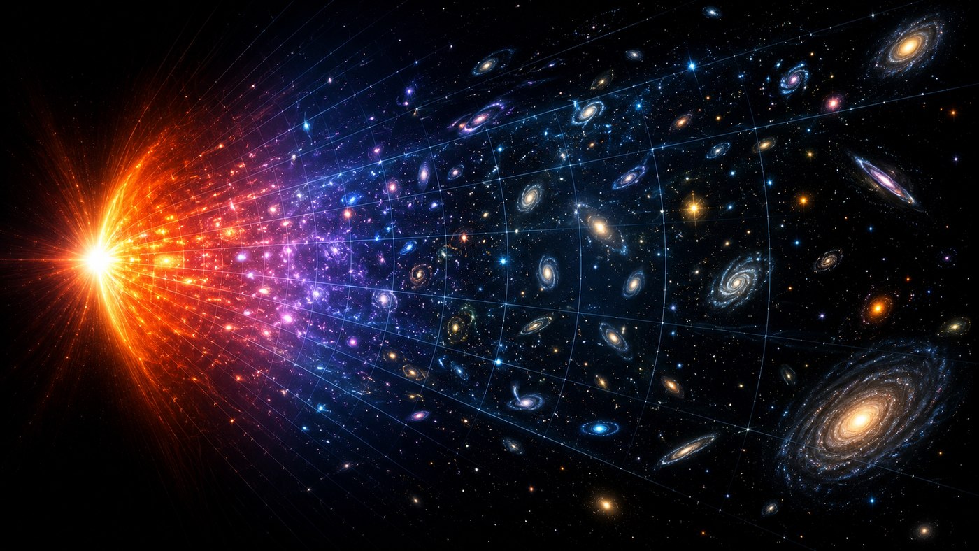
This virtual black hole is nearly infinitely dense, yet only as dense as the total mass and energy of the expanding universe. There is no true singularity in it; there is a defined quantity, set by the contents of the universe. This is the framework’s bounded maximum density (Section 10.5), stated geometrically rather than dynamically.

The entropy between the two states is conserved in the two-sector sense of Section 10.3: as one state approaches its maximum density, it seeds the start of expansion in the other. The expansion can even appear unbounded — an apparently infinite universe — while actually being bounded by the virtual black hole. (Section 10.1 records the precise mathematical cousin of that claim: the de Sitter horizon, with its Gibbons–Hawking temperature and area entropy.)

On this picture the apparent age of the universe is not an absolute statement. The process is continuous — a closed loop rather than a one-time event — and an observer’s “age of the universe” is their position along the cycle. I state this carefully, because its careless form is exactly the claim that killed classical steady-state theory: Section 10.9 records that verdict, and Section 12.7 gives the defensible version — the loop is steady as a geometric object, while epochs, the CMB, and nucleosynthesis remain entirely real. The energy of radiation dissipates as a fourth-power function, appearing as the cooling recorded in the cosmic microwave background (Section 10.6). Gravitational redshift is still present, as is cosmological redshift. What is really different is the boundary: this is a closed system, but not a naive collapsing universe that returns to an infinitely dense starting point.

Virtual space and real space interact in a closed loop. This aligns with the conjecture of Section 3.2 — that pairs of particles flickering in and out of existence are closer to becoming real in some parts of spacetime than others, notably near massive objects. Near maximum compression the vacuum sector is at its densest and most convertible; from our side, that sector is seen simply as the energy present in a vacuum. The point of maximum compression is what we describe as the starting point of expansion: energy, density, and pressure at their highest values — everything that would appear, and be described, exactly like a big bang. But it is a loop, not a one-time process: the expansion energy is balanced by the energy of the virtual sector, and a pressure driving space to expand and increase in entropy has an opposite state in which entropy decreases and density grows in virtual space. I like to describe this with an analogy to chemical reactions — the analogy that seeded this entire framework, recorded in my 2014 notebook and developed in Section 13.

The inside picture carries one geometric difficulty I could never resolve, and I record it because it is what forced the next subsection: I could not really see how a universe many billions of light-years across fits within the black hole. Popławski’s bounce answers this with torsion physics at densities we cannot test. My own answer changed the geometry instead.

STATUS — Conjecture, with published cousins. The two-sector exchange is the conjecture of this whole document; the inside picture is one geometric reading of it. Its mathematical cousins are the de Sitter horizon (Section 10.1), the two-sector universes (Section 10.3), and the bounded maximum density (Section 10.5). Its danger is the steady-state trap (Section 10.9), which the phase-portrait form (Section 12.7) is built to avoid.

7.2 Possible Orbital Shapes of the Universe

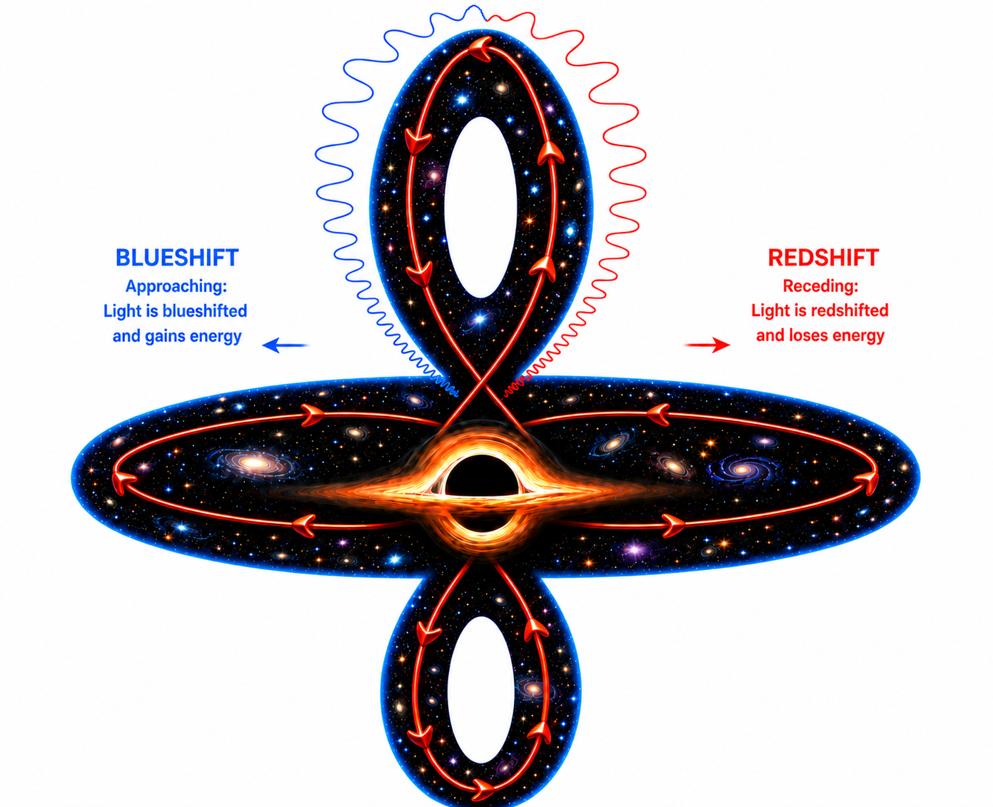
The rectification came, once again, from chemistry. What if, rather than being inside the virtual black hole, we are orbiting it? An atom is mostly empty space: a tiny, dense nucleus with much lighter material occupying an enormously larger volume around it. The orbital shapes could even be like electron orbitals — not planetary circles, but the quantum wavefunctions described by the Schrödinger equation. On this picture the universe is the light material, in a vast orbital, around a supermassive but relatively compact virtual black hole. And black holes are demonstrably not one-way sinks: they are observed to emit streams of light and matter as they absorb new material — Section 7.3 records the sharpest recent case.

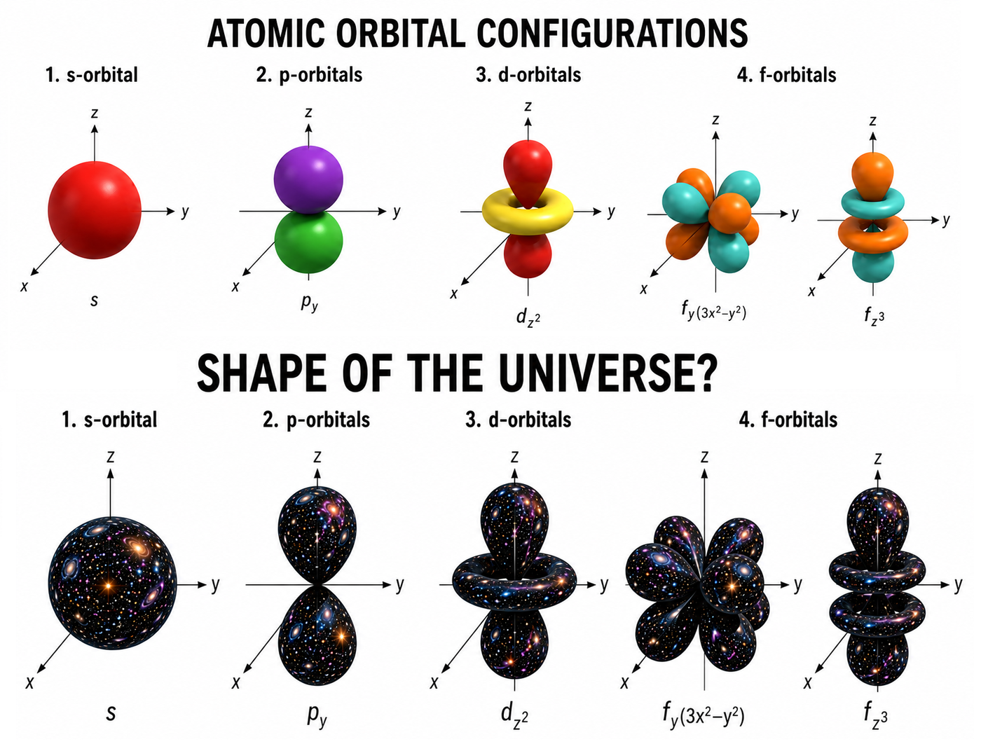
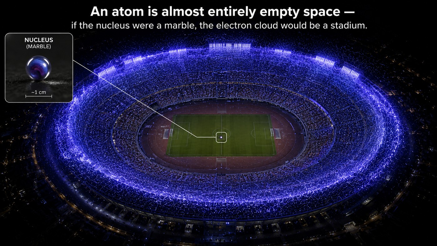
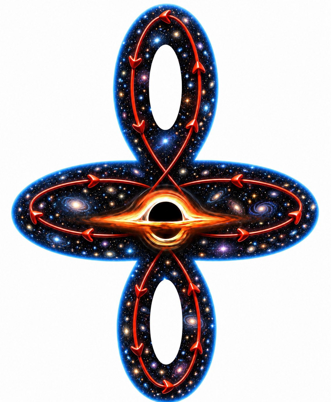
The energy round trip. The key is what an orbit does to energy. As matter and light climb away from the central mass they are redshifted — they lose energy as measured from the starting point. On the return leg they are blueshifted, and on arriving back they are at exactly their original energy, with no loss. In a static gravitational field this is not a conjecture; it is established physics: gravitational red- and blueshift are conservative, and a photon completing a closed path in a stationary spacetime returns at precisely its original frequency. This addresses a famous bookkeeping question head-on — where does the energy “lost” to redshift go? In the closed loop it is not lost. It is stored in the dynamics of the cycle and repaid in full on the inbound leg, which is exactly how cyclic cosmologies treat it: during a contraction phase, every photon blueshifts back. If the loop closes, there is no heat death, no beginning, and no end — the conclusion this document has been driving toward since Section 1.

The constraint any literal orbit must face. An orbit has a direction — toward the center — and a direction is exactly what the sky does not show. The cosmic microwave background is uniform to about one part in 100,000 in every direction once our own motion of roughly 370 km/s is subtracted, and dedicated analyses place tight limits on any preferred axis in the expansion (Saadeh et al., 2016). Nor can orbital Doppler shift replace cosmological redshift: the Hubble law, its isotropy, and the measured (1+z) stretching of supernova light curves (Section 11, item 3) require expansion. So I state the honest form of the claim: any orbital or rotational motion of the universe rides on top of the expansion and must be slow enough to hide beneath the isotropy bounds. It does not substitute for expansion — the mistake that would put this section into the graveyard of Section 10.9.

The published counterpart that keeps the literal version alive. Rotating universes are respectable general relativity: Gödel constructed an exact rotating solution of Einstein’s equations in 1949. And the idea is newly live. In 2025, Szigeti, Szapudi, and collaborators showed that a Gödel-inspired, slowly rotating variant of the standard model resolves the Hubble tension — the persistent disagreement between local and early-universe measurements of the expansion rate — with a rotation so slow, of order one turn per several hundred billion years, that it hides beneath every current measurement (Szigeti et al., 2025). Curiously, the required rate is close to the maximum rotation that avoids closed time-like loops. There are also contested claims pointing the same direction: reported asymmetries in the spin directions of galaxies across the sky (Shamir, 2025), and a contested dipole in the cosmic acceleration itself (Colin et al., 2019). None of this is confirmation. But it means a slow global rotation is a live, published, testable possibility — and it gives the orbital picture its first concrete payoff: if the universe turns, the Hubble tension is where the turning first pays rent.

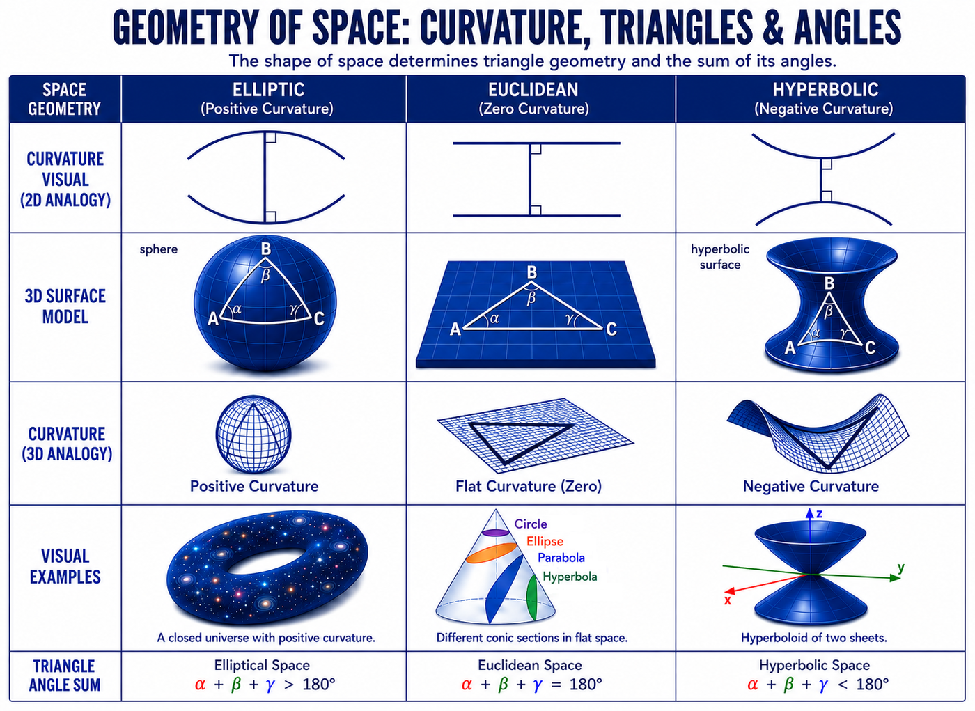
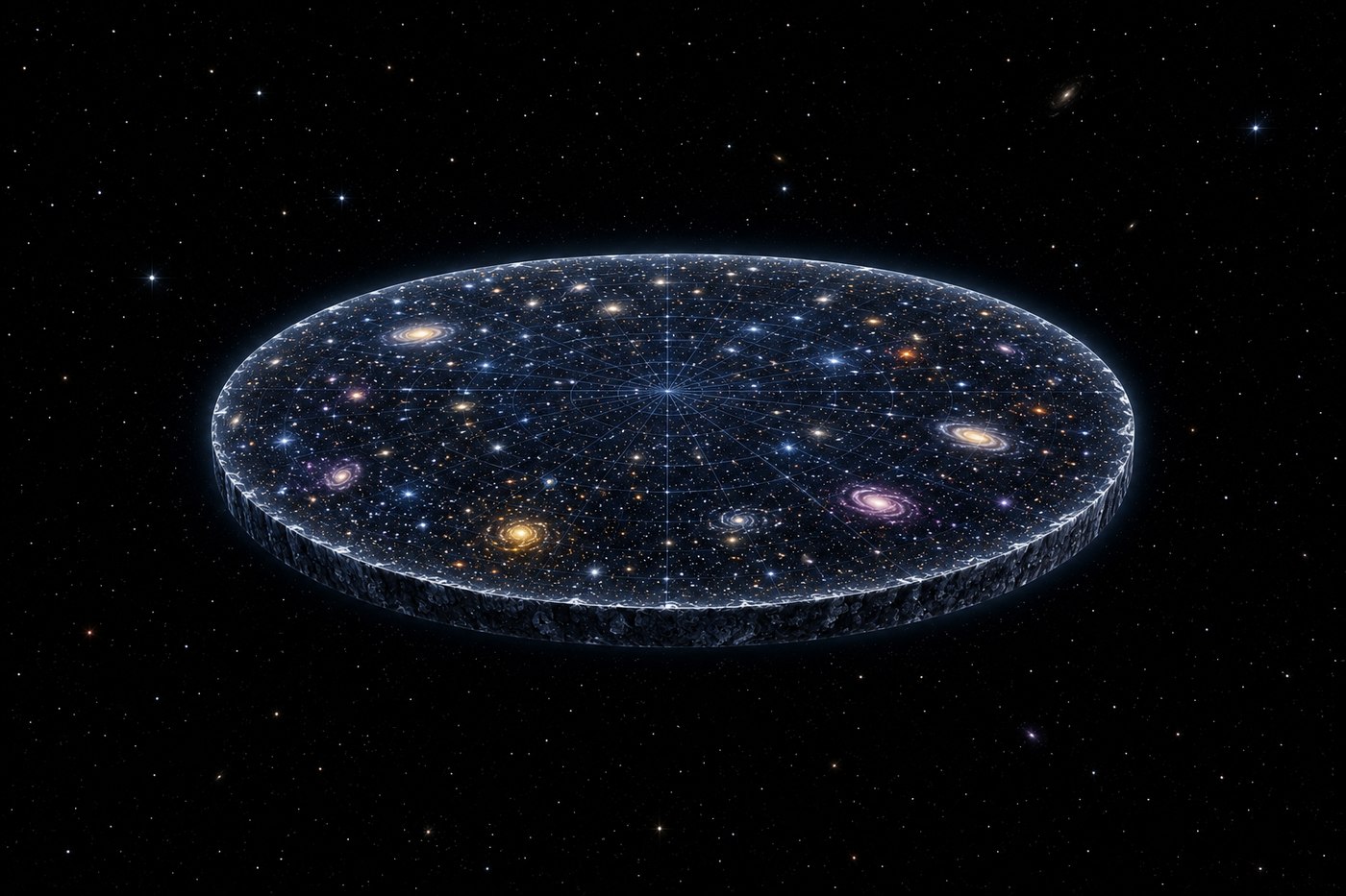
Flat, yet closed. One objection I anticipated: would an orbit not require a closed, curved universe, when we measure flat? No — measured flatness constrains curvature, not topology. A flat 3-torus is a real geometry in which light travels perfectly straight everywhere, every curvature measurement returns zero, and yet space closes back on itself: travel far enough in a straight line and you return to where you began. Searches for the matched-circle signatures such a topology would print on the CMB have found none (Planck Collaboration, 2016), which bounds the size of any such loop to be larger than the observable patch — it does not rule the loop out. “We measure flat, yet the universe loops” is an open possibility, not a contradiction.

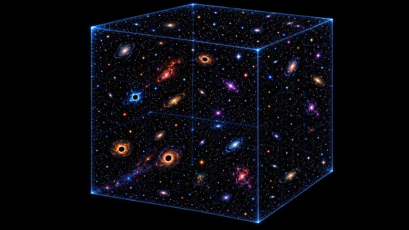
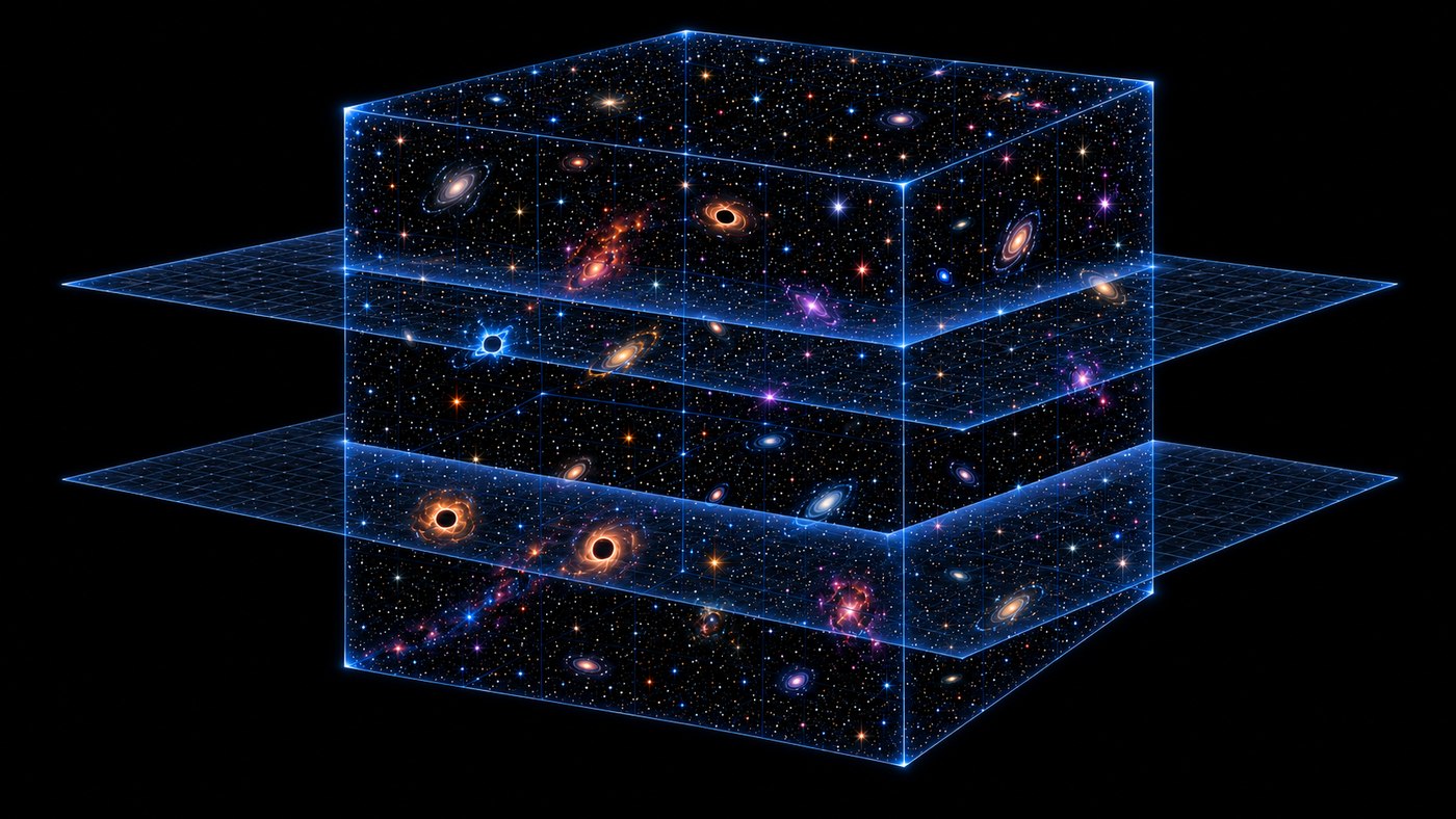
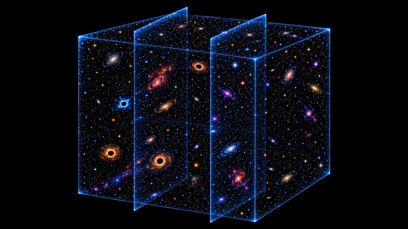
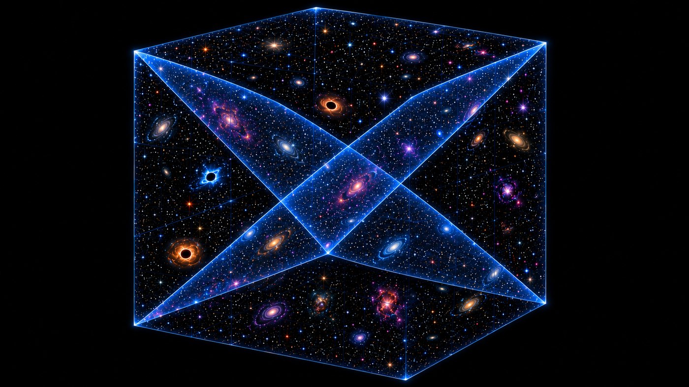
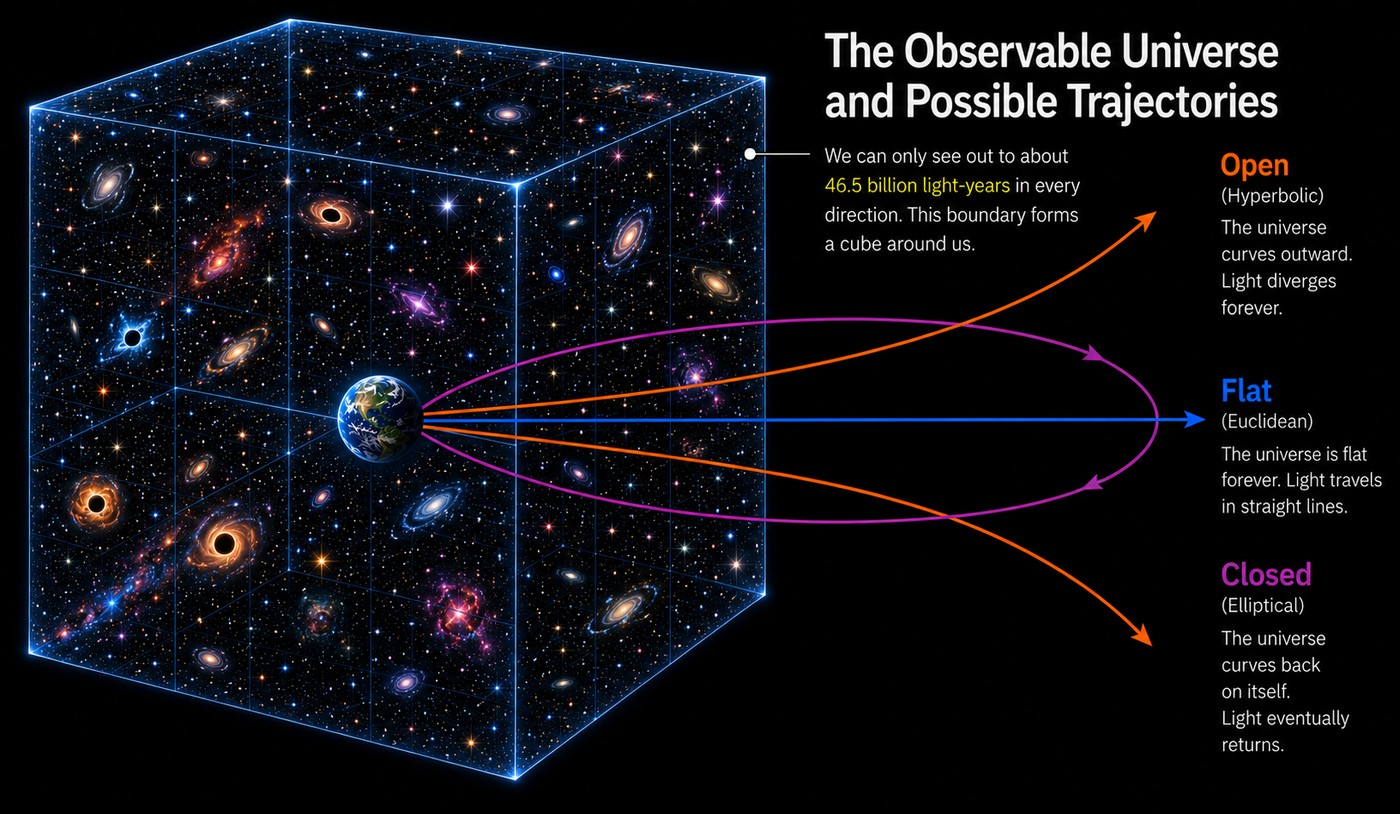
The orbit in state space. The quietest and strongest version of the orbit, though, has been in this document all along. Figure 3(a) already draws the framework’s universe as a literal closed orbit — in state space, size against expansion rate — with no beginning, no end, and “age” reduced to phase along the cycle. The Schrödinger instinct finds its exact, published home there. Quantum cosmology treats the size of the universe as a coordinate moving in a potential and writes a wave equation for it — the Wheeler–DeWitt equation (DeWitt, 1967) — whose famous solutions are precisely “wavefunctions of the universe” (Hartle and Hawking, 1983). Mathematically it is the same species of problem as the hydrogen atom: a wave equation in a potential well, whose solutions are orbitals. Loop quantum cosmology — already this document’s source for the density cap (Sections 10.5 and 12.6) — quantizes exactly this, and the bounce falls out of the quantization. The machinery is rigorous and published; my conjecture is only the identification of that orbit with the two-sector exchange. The orbital picture therefore comes in two strengths: the vivid, vulnerable version — the universe physically circling a central mass — alive only beneath the isotropy bounds, with the slow-rotation model as its foothold; and the state-space version, already drawn in Figure 3(a), whose quantized orbitals are standard quantum cosmology.

One correction the framework accepts. A closed loop must also survive the classical entropy objection: Tolman showed in 1934 that a cyclic universe accumulating entropy cycle over cycle has ever-lengthening cycles, which smuggles a beginning back in. The framework’s answer is the one it already adopted in Section 10.3 — two sectors with opposed arrows of time, each increasing its own entropy along its own arrow. And I keep the two ledgers separate on purpose: the round-trip recovery above balances energy, not entropy. A quantitative version of the entropy ledger remains owed (Section 12.8 lists the debts).

STATUS — Conjecture with published counterparts on both flanks. The slowly rotating universe is peer-reviewed and unconfirmed; the isotropy bounds are the hard constraint any literal orbit lives under; the quantized state-space orbit is standard quantum cosmology whose identification with my two-sector exchange is the conjecture. I now favor this picture over the inside picture of 7.1, while keeping both on the table as geometric realizations of the same exchange.

7.3 Centripetal Acceleration in an Orbit

If the universe is in orbit, the physics of orbital acceleration — especially for light — becomes central, and it holds a surprise that fits this framework unusually well.

Light in a ring. Does light traveling in a ring have centripetal acceleration? Kinematically, yes. Acceleration is any change in velocity, and velocity is a vector: changing direction counts even at constant speed. Light guided around a one-metre ring changes direction continuously, with centripetal magnitude c²/r — about 9×10¹⁶ m/s², roughly 10¹⁶ g. The light carries momentum (p = E/c), and bending its path means redirecting that momentum; the mirrors or fiber absorb the recoil as a real, outward radiation-pressure force, like a track wall pushing back on a cornering car. And because centripetal acceleration is perpendicular to the motion, it does no work: the light’s frequency — its energy — is unchanged. Only the direction turns.

Light orbiting a black hole. Here is the twist that matters. At the photon sphere of a black hole — one and a half times the Schwarzschild radius — light travels in a perfect circle, yet in general relativity its proper acceleration is zero. It follows a geodesic, the straightest possible path through curved spacetime, in free fall the entire way; an ideal accelerometer riding along would read nothing. The circle is only a circle from the outside. And this is no longer theory alone: the Event Horizon Telescope has photographed the ring of light orbiting M87* and Sagittarius A* — light in orbit, observed. The one-sentence summary I will defend: light bent by matter is genuinely accelerating; light bent by gravity only looks like it is — the light travels straight, and spacetime is what is curved. Which raises the framework’s question: if the light is not accelerating, what is? Spacetime is what carries the acceleration.

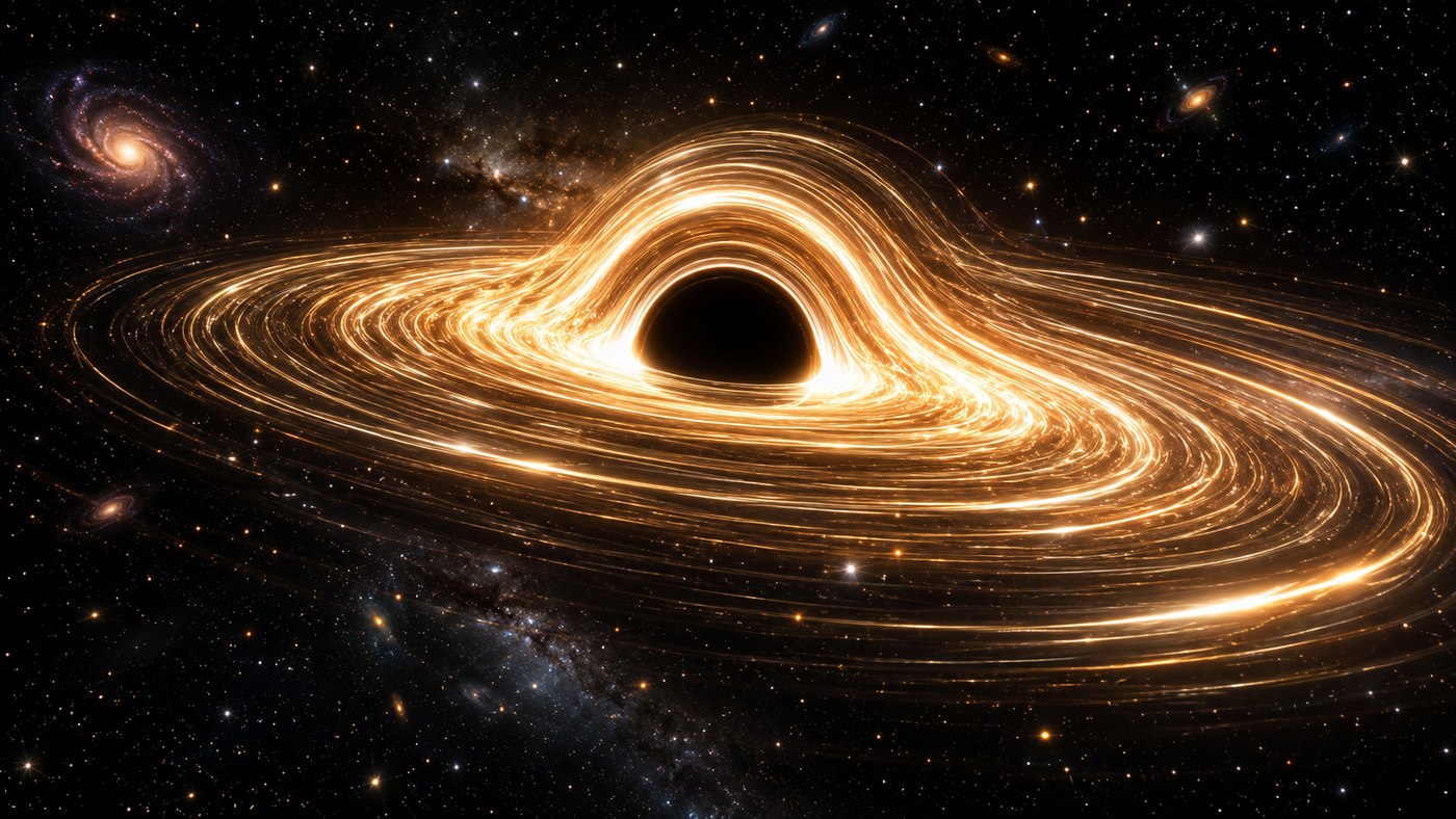
Spacetime itself accelerates — and this is measured. That is not a metaphor; it is frame dragging. Around a rotating mass, spacetime is dragged into co-rotation — the Lense–Thirring effect, measured for the Earth by Gravity Probe B (Everitt et al., 2011). Around a rotating black hole the dragging becomes absolute inside the ergosphere, where nothing can stand still because spacetime itself rotates. And established astrophysics extracts work from this: the Blandford–Znajek mechanism (1977), the leading account of black-hole jets, draws its power from the rotation of spacetime around the hole. This is the closest thing confirmed physics has to the framework’s central instinct — the structure and motion of spacetime doing work.

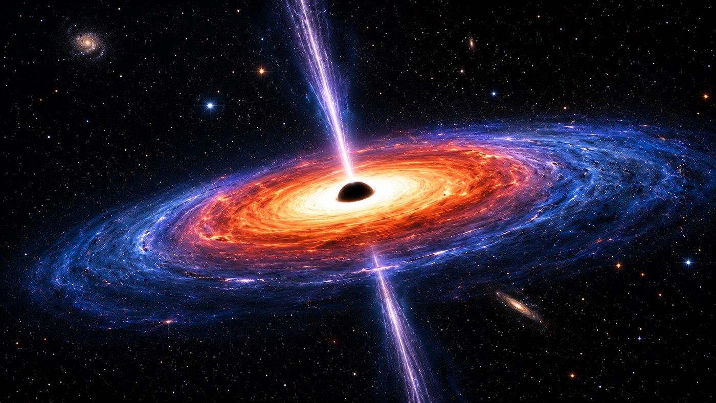
The observed case: a black hole that absorbs and emits. In 2022, astronomers caught a supermassive black hole in the act of devouring a star — the tidal disruption event AT 2022cmc. As it fed, at roughly half a solar mass per year, it launched a jet of matter at 99.99 percent of the speed of light, appearing brighter than a thousand trillion suns because the jet points nearly at Earth (Pasham et al., 2023). I state its meaning for this framework carefully. The jet’s power source is accretion plus, most likely, Blandford–Znajek extraction of the hole’s spin — established astrophysics, not vacuum conversion; nothing in this observation requires my framework. What it demonstrates is the behavior the orbital picture assumes: black holes are not one-way sinks. Absorb-then-emit — infall powering directed outflow, part of the power drawn from spacetime’s own rotation — is observed, spectacular, and routine physics at the center of the picture.

The tie back to the engine: acceleration converts the vacuum. Section 3.1 established that the dynamic Casimir effect, the Unruh effect, and Hawking radiation are three faces of one mechanism: a boundary or observer that is accelerated, or a spacetime that changes, converts vacuum fluctuations into real particles. The Unruh effect has a circular version, and it is the load-bearing fact of this subsection: an observer in circular — centripetal — acceleration sees the vacuum as an approximately thermal bath (Bell and Leinaas, 1983), with a claimed laboratory manifestation in the spin polarization of electrons circulating in storage rings. So orbital acceleration is not merely compatible with the framework’s conversion mechanism; it is an instance of it. If the contents of the universe carry a universal orbital acceleration, that acceleration is itself a vacuum-conversion condition. The chain is: orbit → acceleration → conversion — the conversion term Q of Section 12.2 acquiring, for the first time, a candidate geometric origin.

Could the accelerated expansion be orbital acceleration? I offer this as the subsection’s conjecture, with its caveat and its bridge stated in the same breath. The caveat: the observed cosmic acceleration is isotropic and is an acceleration of the scale factor — every distant galaxy, in every direction, equally — while orbital acceleration points toward a center. A naive identification therefore predicts an anisotropy we do not observe; the contested claims of a dipole in the acceleration (Colin et al., 2019) are exactly the signature to watch, and their fate will constrain this conjecture directly. The bridge, which I regard as the most valuable single number in this section: galactic orbits misbehave — the dark-matter anomaly — below a specific acceleration, a₀ ≈ 1.2×10⁻¹⁰ m/s² (Milgrom, 1983), and that acceleration is numerically about cH₀/2π, the acceleration scale set by the cosmic horizon itself. The scale at which orbital dynamics goes anomalous in galaxies is the scale of the cosmic expansion. That coincidence is published, quantitative, and unexplained; Verlinde’s emergent gravity (Section 10.2) is built on it, and Section 6 now turns on this hinge.

STATUS — Established physics assembled; conjectural identification. Ring light, the photon sphere and its imaging, frame dragging, Blandford–Znajek jets, and the circular Unruh discussion are established or published physics. The identification of cosmic acceleration with orbital acceleration is my conjecture, constrained by isotropy; the a₀ ≈ cH₀/2π coincidence is real and unexplained, and my reading of it is untested.

8. Summary: Where Modern Cosmology Has Gaps, and How This Could Speak to Them

I want to gather the open problems in one place and state, honestly, how my framework relates to each. I claim contact with these questions, not final answers.

The initial singularity.

Cosmology admits this is where the theory breaks. My framework proposes a way for mass present to be a defined quantity and explains why rather than going to infinity.

What dark energy is.

Unknown. I propose it is a property of spacetime structure, matching the geometric role of the cosmological constant in Einstein’s equations.

Whether dark energy evolves.

Actively contested (DESI, ~2.8–4.2 sigma). My framework predicts the static-constant picture is incomplete — the direction the newest data leans. This is my most testable point.

The Hubble tension.

Local and early-universe measurements of the expansion rate disagree at high significance. The orbital picture’s closest published cousin — a slowly rotating universe (Szigeti et al., 2025) — resolves the tension within current bounds. If the framework’s orbit is physical, this is where it first pays rent.

The vacuum-energy catastrophe (120 orders of magnitude).

Unsolved. My framework sits on this question; I conjecture the resolution involves how spacetime structure couples to vacuum energy. We should try to apply numbers to the energy present to match expansion.

The matter–antimatter asymmetry.

Unexplained. Currently, asymmetry-generating processes are what allow real matter to exist at all. It is kind of strange that when matter and antimatter interact they annihilate each other, releasing light — basically creating pure entropy. The result would then quickly be a steady-state heat death of any initial energy. So this occurs near the very dense regions of initial expansion. In less dense regions, spacetime has pairs of particles not emitting light, but the energy is there. Maybe this interaction of particles could be a reason for gravity or dark energy — the thought Section 6 now develops. What is the exact force of particles coming in and out of existence, and what does this energy balance look like? It would be worth exploring.

Dark matter.

Unknown composition. I now conjecture (Section 6) that dark matter is the gravitating weight of the vacuum sector — the mass of pairs coming in and out of existence, modulated by local spacetime structure — anchored by the published coincidence that the rotation-curve acceleration scale a₀ matches cH₀/2π. The Bullet Cluster is the test this must pass; the undiscovered-particle explanation remains fully compatible.

Energy accounting across cosmic expansion.

Global energy conservation genuinely loosens in an expanding universe. My “balancing sector” conjecture attempts to restore it; it needs a distinct, falsifiable prediction to become physics. It needs to show the mechanism for how it loops back.

9. What This Framework Still Needs

I hold this outline to the same standard I would hold anyone else’s. A picture becomes a theory when it produces a number that could be measured and found wrong. My framework’s components touch real, respected physics — the dynamic Casimir effect, gravitational particle production, the geometric cosmological constant, evolving dark energy, redshift, and bounce cosmology. What it still lacks is the connective mathematics that turns the picture into specific predictions that differ from the standard model’s.

The honest next step is to take the single most testable claim — that dark energy evolves in a specific way — and derive, from the framework, a rule for how the expansion rate should change over time, then lay that rule against the DESI reconstruction and let it succeed or fail. That is the move that would turn this from an interpretation into a candidate theory. Until then, I present it as what it is: a coherent conjecture, built from real phenomena, aimed at the genuine open questions of cosmology. A second data-facing descendant now exists as well: if the orbital picture of Section 7.2 is physical, its slow global rotation speaks to the Hubble tension, and the rotation rate is a second number the framework must eventually pin down.

10. Published Counterparts

Ideas do not earn credibility in isolation; they earn it by contact with work that has survived peer review. This section collects the published physics that each piece of my framework corresponds to — the real counterparts of my conjectures. For each one I state what the published result says, how it maps onto my picture, and what its standing is. Some of these counterparts strengthen my framework. One of them — the fate of classical steady-state theory — is a warning I take seriously and record here on purpose.

10.1 Horizon Thermodynamics: The De Sitter Horizon as the “Virtual Black Hole”

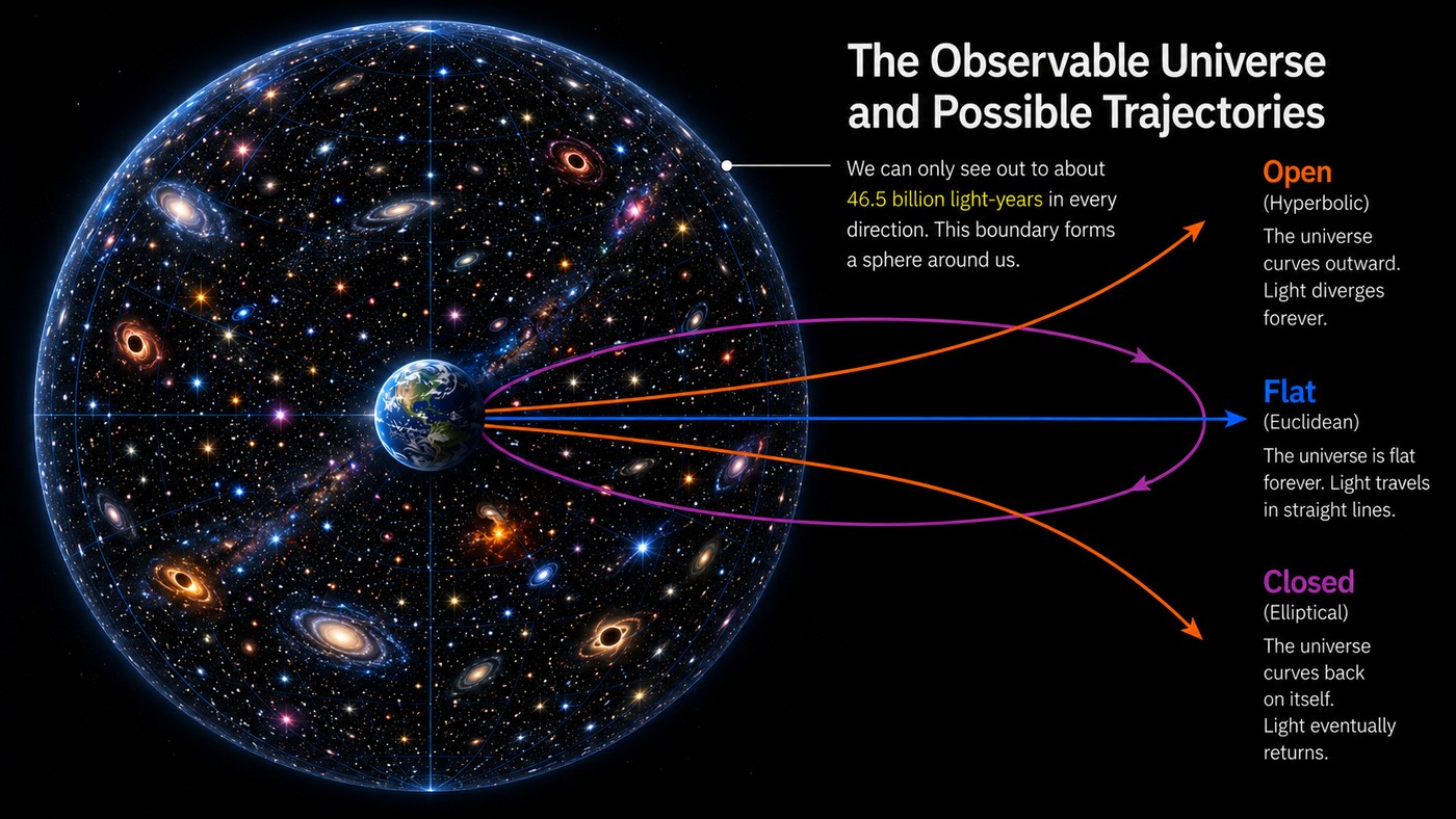
My “virtual black hole that is the opposite of expansion” (Section 7.1) has a precise mathematical cousin. Gibbons and Hawking showed in 1977 that an accelerating universe possesses a cosmological event horizon that behaves like an inside-out black hole: it has a temperature and an entropy proportional to its area, exactly as a black hole horizon does. Every observer in a dark-energy-dominated universe lives inside such a horizon, which bounds what they can ever see. The related holographic entropy bounds (Bekenstein; Bousso) state that the maximum entropy of a region is set by the area of its boundary — a rigorous version of my claim that the expansion “can appear infinite but is actually bounded by the virtual black hole.” There is also a suggestive numerical coincidence: the Schwarzschild radius computed for the mass-energy of the observable universe is roughly the size of the observable universe itself, a consequence of the universe sitting near critical density — the same coincidence that motivates black-hole-cosmology proposals like the one in Section 7.

One update, now that Section 7 holds two geometries. The Gibbons–Hawking horizon is the exact mathematical cousin of the inside picture (Section 7.1): the virtual black hole as a boundary surrounding every observer. The orbital picture (Section 7.2), which I now favor, has different cousins — Gödel’s rotating solution and the modern slow-rotation models — while the horizon physics recorded here remains standing, established physics on either reading. The two identifications are alternatives, and I keep both flagged.

STATUS — Established (the physics); Conjecture (my identification). De Sitter horizon temperature and entropy, and holographic bounds, are standard results. My move — identifying this horizon structure with the “virtual” sector of my framework — is the conjecture, not the horizon physics itself.

10.2 Gravity as Thermodynamics of the Vacuum (Jacobson, Padmanabhan, Verlinde)

The deepest published counterpart to my central instinct — that spacetime structure and vacuum energy are two faces of one thing — is thermodynamic gravity. In 1995 Ted Jacobson derived the Einstein field equations from the thermodynamics of local horizons plus the entropy-area law, treating gravity as an equation of state of the vacuum rather than a fundamental force. Padmanabhan extended this program, and Verlinde proposed that gravity is emergent and entropic, even claiming that dark-matter-like effects can arise from vacuum entropy — which is now the published counterpart of my dark-matter conjecture in Section 6. If my framework is to acquire a mathematical spine, this lineage is where it lives.

STATUS — Established derivation; interpretation actively debated. Jacobson’s derivation is accepted mathematics and widely cited. Whether it means gravity is “really” thermodynamic — and whether Verlinde’s dark-matter extension survives observational tests — remains contested. It is nevertheless a live, respected research program built on exactly my unifying instinct.

10.3 Two-Sector and Mirror Universes (Boyle–Finn–Turok; Aguirre–Gratton)

My proposal that the real expanding sector is balanced by a complementary sector, so that the global books close, has a striking peer-reviewed counterpart: the CPT-symmetric universe of Boyle, Finn, and Turok (2018). There, the Big Bang is a mirror surface, and the “other side” is an anti-universe running with time reversed, so that the universe-plus-mirror pair conserves charge, parity, and time symmetry globally. Aguirre and Gratton’s steady-state eternal inflation similarly builds a spacetime with two arrows of time growing out of a middle slice. These models also contain the standard repair for my entropy bookkeeping: entropy increases in both sectors along their own arrows of time, which point away from each other — making “entropy is conserved between the states” coherent without violating the second law in either sector.

STATUS — Conjecture with published counterparts. Both models are peer-reviewed, mathematically developed, and minority views. Neither is confirmed. They demonstrate that my two-sector move is a legitimate theoretical strategy, not a category error — and they show the specific mechanism (opposed arrows of time) my framework should adopt.

10.4 The Zero-Energy Universe (Tryon; Hawking)

My bedrock commitment — that nothing is ever created from nothing and the global books must balance — has a home in the zero-energy universe hypothesis. Tryon proposed in 1973 that the positive energy of all matter may be exactly canceled by the negative gravitational binding energy of the universe, so that the total is zero; Hawking popularized the same accounting. On this view the universe never required an energy deposit at all: the books were never opened. This is the published version of my “conservation, not creation” principle applied at cosmic scale, and it coexists naturally with the loosening of global energy conservation in expanding spacetime discussed in Section 5.

STATUS — Open problem / published hypothesis. Defining total energy in general relativity is subtle, and the zero-energy claim depends on the definition used. It is not established, but it is a serious, frequently cited idea that shares my framework’s core commitment.

10.5 Bounded Maximum Density Instead of a Singularity

My claim that the “virtual black hole” is not a true singularity but only as dense as the mass-energy of the universe corresponds to the limiting-curvature hypothesis (Markov) and its modern descendants. In loop quantum cosmology, the bounce occurs when density reaches a finite maximum of order the Planck density — the singularity is replaced by a cap. Rovelli and Vidotto’s Planck stars apply the same idea to black hole interiors. Popławski’s torsion bounce (Section 7) achieves the same end through a different mechanism. All of these share my framework’s structural feature: a defined, finite maximum density set by physics, in place of the infinite-density origin I object to in Section 1.

STATUS — Conjecture, active research. None of these bounce mechanisms has been tested — the required physics lies at densities we cannot probe. But they are mathematically developed, published programs, and they establish that “finite cap, not singularity” is a respectable position.

10.6 The Fourth-Power Dissipation of Radiation

I wrote that the energy of light dissipates as a fourth-order function, appearing as the cooling we observe in the cosmic background radiation. Standard cosmology contains exactly this law: radiation energy density dilutes as the fourth power of the scale factor — three powers from the growth of volume and one more because expansion stretches each photon to lower energy. The cosmic microwave background’s temperature falls in precisely this way. My intuition matches the established scaling.

STATUS — Established — with a double edge. The fourth-power law is textbook physics. The edge: this same scaling has been measured directly at high redshift (the CMB temperature at earlier epochs, read from molecular clouds, follows T(z) = T₀(1+z)), which proves the universe genuinely was hotter and denser in the past — everywhere. That measurement supports my dissipation claim while directly pressuring my “apparent age” claim; see 10.9.

10.7 Cosmologically Coupled Black Holes (Farrah et al., 2023)

My conjecture in Section 3.1 — that black holes might gain mass because spacetime structure converts vacuum into real particles within them — has a published, observational cousin that I record here as a case study. In 2023, Farrah and collaborators claimed evidence that black holes gain mass through “cosmological coupling” to the expansion of the universe itself, and even proposed that black holes could be the source of dark energy. The claim was peer-reviewed, made headlines, and was then largely dismantled by follow-up work: independent samples failed to reproduce the coupling, and the growth of supermassive black holes is well accounted for by ordinary accretion — the Soltan argument ties the total light emitted by quasars over cosmic history to the black hole mass we observe today, and the budget balances. I also note the theoretical obstacle to my version: in a stationary spacetime, the time symmetry that defines energy conservation forbids spontaneous particle production, which is why Hawking radiation requires a horizon and drains its source.

STATUS — Contested and largely disfavored. This is the closest real-world test of my black-hole-growth conjecture, and the data currently comes down against it. I keep the conjecture flagged as such in Section 3.1, and I record this counterpart deliberately: it shows what happens when exactly this intuition meets observation.

10.8 Interacting Dark Energy and Phantom Crossing (The DESI Connection)

This is the counterpart that matters most, because it points to my framework’s concrete next step. There is an established literature of “interacting dark energy” models, in which dark energy exchanges energy with another sector through an explicit coupling term Q in the Friedmann equations. My vacuum-conversion picture is structurally a model of this class: the conversion between the vacuum sector and the real sector is an energy exchange. The connection to data: the DESI results hint that the dark energy equation of state w crossed the value −1 in the recent past (“phantom crossing”). A single, simple dark-energy field cannot cross that line — but models in which dark energy exchanges energy with another sector can mimic phantom crossing naturally. In other words, if the DESI anomaly is real, it favors precisely the class of models my framework belongs to. The falsifiable move is to write my conversion rate as an explicit exchange term, derive the effective w(z) it produces, and lay it against the DESI-preferred region of parameter space.

STATUS — Open problem — the live frontier. The DESI preference for evolving dark energy stands at roughly 2.8 to 4.2 sigma depending on which supernova sample is combined with it, and Bayesian reanalyses find the evidence weaker still, possibly driven by tensions between datasets. It is genuinely unsettled — which is exactly why a distinct prediction from my framework, laid against this data, is the single most valuable calculation I could produce.

10.9 A Cautionary Counterpart: Classical Steady-State Theory

Honesty requires me to include the published counterpart that failed. My suggestion that the process is continuous and the apparent age of the universe is a matter of our location is a relative of the classical steady-state theory of Hoyle, Bondi, and Gold, which held that the universe looks the same at all epochs. That theory was killed in the 1960s by exactly the observations my picture must now face: the cosmic microwave background and its measured temperature evolution with redshift, the light-element abundances that require a hot dense phase, the visible evolution of galaxies and quasars with lookback time, and the source counts. The universe demonstrably had eras. I draw the lesson explicitly: my framework does not actually need the steady-state claim. A closed-loop conversion cycle is compatible with real epochs — this is how Penrose’s conformal cyclic cosmology and the Steinhardt–Turok cyclic models survive the same evidence. The claims “the process has no beginning” and “the age is only apparent” are separable, and only the second conflicts with observation. I retain the first and place the second under maximum doubt. (Section 12.7 gives the precise sense in which a loop can be called steady: as a closed orbit in state space, not as unchanging observations.)

STATUS — Falsified (as originally stated). Classical steady-state theory is one of cosmology’s clearest examples of a beautiful idea rejected by data. Recording it here is the standard I set in the preface: the framework must be judged against the strongest evidence, including the evidence against its relatives.

11. What Any Candidate Theory Must Reproduce

A unified field theory must reconcile general relativity with quantum mechanics, ideally yielding governing equations — as Maxwell unified electricity and magnetism, and as Dirac partially unified special relativity with quantum mechanics, predicting antimatter in the process. By that standard, this draft is a cosmological hypothesis, not yet a unified field theory, and I say so plainly. What follows is the checklist of observations any serious candidate has to fit. The standard model of cosmology fits all of them, with known tensions; a challenger must do at least as well before any of its advantages count.

1. The cosmic microwave background. The blackbody spectrum (2.725 K, deviations below 50 parts per million), the acoustic power spectrum of its fluctuations, and its measured temperature evolution with redshift, T(z) = T₀(1+z) — the observation that established that the universe genuinely had hotter, denser epochs (see 10.9).

2. Primordial light-element abundances. Roughly 75% hydrogen and 25% helium-4 by mass, plus trace deuterium and lithium, as produced in a hot dense phase. (The lithium abundance carries a known tension even in the standard model — a challenger that resolved it would score a genuine point.)

3. The redshift–distance relation and time dilation. The Hubble law, and the observed (1+z) stretching of supernova light curves — direct evidence that cosmological redshift is expansion, not tired light.

4. Baryon acoustic oscillations and structure growth. The BAO standard ruler measured across redshift (the DESI data itself), and the growth history of large-scale structure. Any modification I make to the dark-energy sector is tested here first.

5. The dark-matter suite. Galaxy rotation curves, gravitational lensing, the CMB peak structure, and the Bullet Cluster, where the gravitating mass demonstrably separates from the visible gas.

6. The accelerating expansion. The Type Ia supernova result and its concordance with the CMB and BAO — the dark-energy observation my framework most directly addresses.

7. Black-hole observations. Merger waveforms (LIGO/Virgo), horizon-scale imaging (Event Horizon Telescope), and the multimessenger constraint that gravitational waves travel at the speed of light to within one part in 10¹⁵ (GW170817), which has already eliminated whole families of modified-gravity theories.

8. Local relativity and equivalence-principle tests. Gravitational time dilation, perihelion precession, light bending, the Shapiro delay — and the equivalence principle itself, tested to parts in 10¹⁵ (MICROSCOPE). My conjecture that particle creation is “cheaper” in some locations must survive this bound or confine itself to regimes these experiments cannot reach.

9. Precision tests of the quantum vacuum. The electron’s magnetic moment agrees with vacuum-fluctuation theory to roughly twelve digits, and the Lamb shift and static Casimir force are measured to match. A framework in which the vacuum converts to real particles must leave these numbers untouched — the vacuum is the most precisely tested object in physics, and any new conversion channel must be utterly negligible in the laboratory.

10. Singularity handling. A resolution, or controlled handling, of the singularities at black-hole centres and at the apparent beginning — replacing infinities with finite, defined quantities, as my framework proposes.

11. The matter–antimatter asymmetry. An account of why any matter survived annihilation — the origin of the surplus we are made of.

12. Internal consistency. A conserved total energy ledger across the real and virtual sectors, with an explicit mechanism for how the loop closes — the requirement I set for my own “balancing sector” in Section 8.

A practical strategy follows from this list, and I want to state it with the tradeoff exposed. The singularity problem (item 10) is where my framework is most distinctive — a virtual-sector exchange could in principle cap densities at a finite value — but it is also the least testable item on the list, because no observation can currently reach that regime; a calculation there can be interesting but cannot yet be wrong. The evolving-dark-energy question (items 4 and 6) is the reverse: less distinctive, but facing live data today. So the order of operations is: first, derive the exchange-term prediction for w(z) and lay it against the DESI reconstruction, because falsifiability requires data that can answer back; second, develop the density-cap calculation as the framework’s conceptual differentiator. One solid quantitative win is worth more than ten qualitative gestures across the whole list.

STATUS — The bar I accept. Every item above is established observation (with the noted lithium tension). I list them not as decoration but as the standard this framework must meet. Where the framework speaks — items 4, 6, 10, and 12, and now the dark-matter suite through the conjecture of Section 6 — it must eventually produce numbers; where it is silent, it must at minimum not conflict.

12. A First Calculation: The Friedmann Equations with a Conversion Term

Sections 9 and 11 both end with the same demand: produce a number. This section carries out the first step. I write the standard equations governing cosmic expansion, then the updated version containing my framework’s conversion term, then I solve two concrete examples exactly and lay the results against the DESI measurements. The examples were verified by direct numerical integration of the coupled equations.

12.1 The Standard Equations

The expansion of the universe is governed by the Friedmann equations. In plain language:

(expansion rate)² = (constant) × (total density) − (curvature term)

(acceleration of expansion) ∝ −(density + 3 × pressure)

In symbols, with a(t) the scale factor and H = (da/dt)/a the expansion rate:

H² = (8πG/3) ρ − k/a² (12.1)

(d²a/dt²)/a = −(4πG/3)(ρ + 3p) (12.2)

The second ingredient is the bookkeeping law. Each energy component, with equation of state w = p/ρ, obeys the continuity equation:

dρ/dt + 3H(1 + w)ρ = 0 (12.3)

Reading the symbols:

a(t) — the “size” of the universe — the stretch factor of space relative to today (a = 1 now; a = 0.5 means everything was half as far apart)

H — the expansion rate — the fractional growth of a per unit time, H = (da/dt)/a; its value today is the Hubble constant H₀

G — Newton’s gravitational constant — the strength of gravity

ρ — (“rho”) the total energy density — matter, radiation, and vacuum energy combined

p — the total pressure exerted by that content

k — the curvature of space — k = 0 flat, k positive closed and finite, k negative open

d/dt — “the rate of change of”; d²a/dt² is the acceleration of the expansion

w — the equation of state — pressure divided by energy density, w = p/ρ; this one number fixes how a component thins out as space grows

z — redshift — light from earlier epochs arrives stretched; a = 1/(1+z), so z = 1 labels the epoch when the universe was half its present size

w₀, wₐ — the standard two-number summary of an evolving w — its value today (w₀) and how strongly it changes back in time (wₐ)

Ωₘ, Ωᵥ — today’s matter and vacuum densities as fractions of the critical density; measured values ≈ 0.31 and 0.69

This single law generates all the standard behaviour. Matter (w = 0) dilutes as a⁻³ with volume. Radiation (w = 1/3) dilutes as a⁻⁴ — the fourth-power law of Section 10.6. A cosmological constant (w = −1) does not dilute at all. The standard model of cosmology, ΛCDM, is exactly these pieces evolving side by side with no exchange between them.

STATUS — Established. The Friedmann and continuity equations follow from general relativity applied to a homogeneous universe and underlie every result cited in this document.

12.2 The Updated Version: Adding the Conversion Term Q

My framework changes nothing in the Friedmann equations themselves — all energy still gravitates, and the expansion still responds to the total. What changes is the bookkeeping. I split the ledger into a real sector (matter, density ρₘ) and a vacuum sector (density ρᵥ, intrinsic equation of state w = −1), and I let them exchange energy at a rate Q:

dρₘ/dt + 3Hρₘ = +Q (real sector) (12.4)

dρᵥ/dt = −Q (vacuum sector) (12.5)

ρₘ — energy density of the real sector — ordinary matter and radiation

ρᵥ — energy density of the vacuum sector

Q — the conversion rate — energy per unit volume per unit time transferred between the sectors; the framework’s single new ingredient

The sign convention: Q greater than zero means the vacuum is converting into real matter and energy; Q less than zero means the real sector is converting back into the vacuum. Adding the two equations shows that the total obeys exact conservation — whatever leaves one sector arrives in the other. The loop closes by construction. This is the explicit mechanism that Section 8 demanded of my “balancing sector,” now written as an equation rather than a sentence.

The key identity, Eq. (12.6), follows immediately. An observer who fits the data with a standard, non-interacting model — which is what every survey does — will attribute the exchange to an evolving dark-energy equation of state:

w(z) = −1 + Q / (3Hρᵥ) (12.6)

Conversion masquerades as dynamics. When the vacuum drains into the real sector (Q positive), the vacuum density falls with time and the observer measures w above −1. When the real sector converts back into the vacuum (Q negative), the vacuum density grows and the observer measures w below −1 — apparent “phantom” behaviour from a model in which nothing exotic exists. This masquerade is a known, published result in the interacting-dark-energy literature (Das, Corasaniti, and Khoury, 2006): coupling between sectors can imitate phantom dark energy without any component ever violating an energy condition.

STATUS — Established machinery; conjectural identification. The coupled equations and the effective-w identity are standard tools of the interacting-dark-energy literature. My conjecture is the identification: that Q is the vacuum-to-real conversion governed by spacetime structure (Section 3), rather than a phenomenological coupling.

12.3 Worked Example A — Conversion at a Constant Fractional Rate

The simplest possible choice: the vacuum converts at a fixed fraction of itself per e-fold of expansion (each factor of e ≈ 2.7 growth in size), Q = 3αHρᵥ, with the dimensionless number α setting that fraction. The coupled equations, Eqs. (12.4)–(12.5), then solve exactly:

ρᵥ(a) = ρᵥ₀ · a^(−3α) → w = −1 + α (constant) (12.7)

ρₘ(a) = [ρₘ₀ − (α/(1−α))ρᵥ₀] · a⁻³ + (α/(1−α))ρᵥ₀ · a^(−3α) (12.8)

With today’s densities Ωₘ = 0.31 and Ωᵥ = 0.69 and a conversion rate of α = 0.1, the vacuum behaves as dark energy with w = −0.90, forever, and was 23% denser at redshift 1 than it is today. The matter sector carries a small extra piece that tracks the vacuum — the accumulated converted material. The verdict is immediate: this model predicts a constant w, so wₐ = 0 exactly. The DESI signal, if real, is concentrated in the evolution of w, not its offset. A constant-rate conversion is therefore already disfavored as the sole story — the first genuinely falsifiable statement the framework has produced, and the data has already spoken on it.

STATUS — Solved exactly; disfavored as the sole mechanism. A useful failure: it demonstrates the machinery works end to end — assumption in, measurable number out, comparison with data. It also proves the framework needs a Q that varies, which Example B and the DESI inversion below supply.

12.4 Worked Example B — Conversion Tied to the Real Sector: Phantom Crossing Appears

Now let the conversion rate track the real sector instead: Q = 3αHρₘ. The equations again solve exactly (I verified both closed forms by direct numerical integration of the coupled system):

ρₘ(a) = ρₘ₀ · a^(−3(1−α)) (12.9)

ρᵥ(a) = ρᵥ₀ + (α/(1−α)) ρₘ₀ · [a^(−3(1−α)) − 1] (12.10)

Matter now dilutes slightly slower than a⁻³, because it is continuously replenished from the vacuum. Here is the subtle and important part. An observer — a real survey — assumes matter dilutes exactly as a⁻³, anchored to today’s value. Everything left over gets called dark energy. Computing the equation of state of that leftover, with α = 0.03, gives:

z = 0: w = −1.000 z = 0.25: w = −1.018 z = 0.5: w = −1.056

z = 0.75: w = −1.126 z = 1.0: w = −1.249

The effective dark energy is phantom (w below −1) in the past and crosses −1 at the present epoch — produced by a model in which no ingredient is phantom, no energy condition is violated, and the total ledger balances exactly. Apparent phantom crossing is the fingerprint of the exchange. Fitting the standard two-parameter form w(z) = w₀ + wₐ·z/(1+z) to the solution of Eqs. (12.9)–(12.10) over 0 < z < 1 gives w₀ = −0.94 and wₐ = −0.45: the same quadrant as the DESI result. Two further honest notes. First, in this model the effective dark-energy density shrinks into the past and passes through zero near z ≈ 2.2 — which connects to a discussion already present in the post-DESI literature of effective dark-energy density going negative at high redshift, and is a reminder that the w₀–wₐ form is a crude wrapper around richer behaviour. Second, the crossing lands at z = 0 here only because the model is anchored to today’s densities; richer forms of Q move it.

STATUS — Solved exactly; reproduces the observed shape. A one-parameter conversion term generates evolving, phantom-crossing dark energy with wₐ < 0 — the qualitative structure of the DESI anomaly — from pure bookkeeping. It does not hit the DESI central values; the next subsection shows what would.

12.5 Reading the DESI Numbers Through the Framework: The Conversion Changed Direction

The DESI DR2 central values, for reference: BAO with CMB alone gives w₀ = −0.42 ± 0.21 and wₐ = −1.75 ± 0.58; adding the Pantheon+ supernovae gives w₀ = −0.838 ± 0.055 and wₐ ≈ −0.62; the DESY5 supernova combination sits near w₀ ≈ −0.75 and wₐ ≈ −0.86. Every combination lands in the same quadrant: w₀ above −1, wₐ below zero. Now run the key identity, Eq. (12.6), backwards. Given a measured w(z), the implied conversion rate is:

Q(z) = 3H(z) ρᵥ(z) · [1 + w(z)] (12.11)

Read this way, the data makes a statement in my framework’s native language. Today, w is above −1, so Q is positive: the vacuum is currently converting into the real sector. In the past, w was below −1, so Q was negative: the real sector was converting into the vacuum. The conversion direction flipped — at z ≈ 0.41 for the DESY5 combination, z ≈ 0.35 for Pantheon+, z ≈ 0.5 for BAO with CMB alone — roughly four to five billion years ago. The magnitude today: the vacuum sector is draining on an e-folding timescale of about 19 to 30 billion years, i.e. roughly 3 to 5 percent of the vacuum per billion years. That rate, translated to laboratory scales, is of order one part in 10¹⁰ per year — utterly invisible to the precision vacuum tests of Section 11, item 9, exactly as required.

This is the payoff of the calculation. The minimal one-parameter models of 12.3 and 12.4 capture the quadrant but not the central values (Figure 1); hitting the central values requires a Q that changes sign over cosmic history. A sign-changing conversion is not an epicycle bolted on — it is the native structure of my closed-loop picture, in which the exchange runs one way in one regime and reverses in the other. And sign-switching interactions between the dark sectors are, post-DESI, an active topic in the published literature. If the DESI anomaly survives (Section 10.8 records why it may not), it is, at face value, the signature of a two-sector exchange that recently reversed direction.

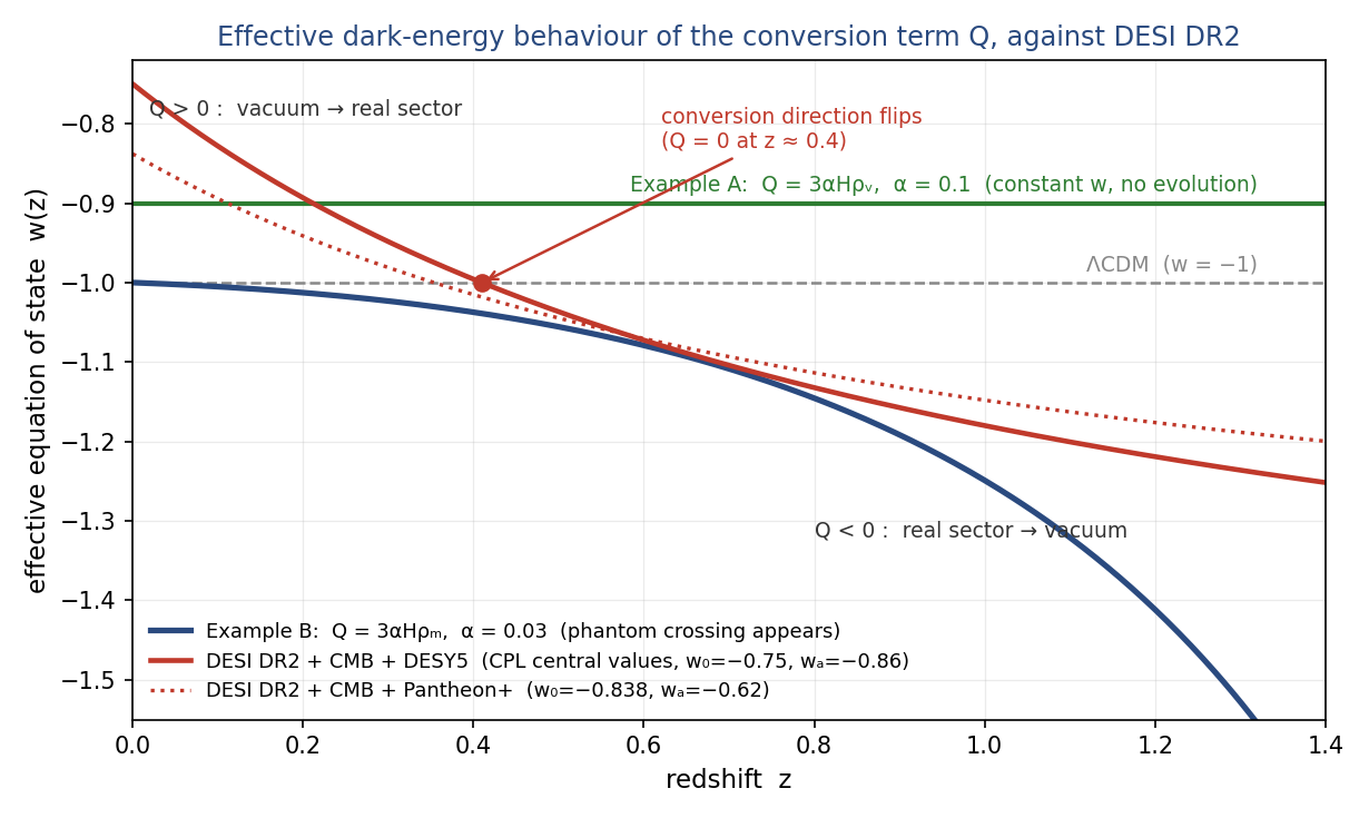
STATUS — The framework’s first quantitative, falsifiable statement. Prediction: if the conversion picture is right, the reconstructed w(z) should continue to show a genuine crossing of −1 near z ≈ 0.4, and the effective dark-energy density should decrease toward higher redshift. Future DESI releases and other Stage-IV surveys can confirm or destroy this. If the anomaly dissolves into supernova systematics, Q is consistent with zero and the framework loses its only current observational support.

12.6 The Fate of the Universe: Runaway, Recollapse, or Closed Loop

Figure 1 shows the engine — how the conversion term appears in the measured equation of state. It does not show the outcome, and the outcome is the question this document opened with. Writing Eq. (12.1) for a universe containing matter, dark energy with any history, and curvature, and dividing through by today’s critical density, gives the master equation for the trajectory:

H² = H₀² · [ Ωₘ a⁻³ + Ω_de · f(a) + Ωₖ a⁻² ] (12.12)

f(a) — the dilution history of dark energy, fixed by w(z); f = 1 for a cosmological constant

Ωₖ — the curvature contribution — zero if space is exactly flat

Every possible fate is a solution of this one equation; only the contents differ. Figure 2 shows four trajectories, integrated numerically. A fixed cosmological constant produces the accelerating runaway — expansion forever, the fate Section 4.1 noted a cyclic picture must escape. The DESI central values, extrapolated forward, produce something genuinely different: because wₐ is negative, the dark-energy density fades away in the future, the acceleration switches off, and the universe coasts. The newest data, taken at face value, already removes the runaway — though, exactly as Section 4.1 was careful to say, it does not by itself produce a reversal. A closed universe without dark energy halts and recollapses, ending in precisely the singularity I rejected in Section 1. The fourth trajectory is the framework’s: the same recollapse, but with the bounded maximum density of Section 10.5 imposed through the published loop-quantum-cosmology correction:

H² → H² · (1 − ρ/ρ_c) (12.13)

ρ_c — the density cap — the finite maximum density at which contraction reverses (Section 10.5)

When the density reaches the cap, the expansion rate passes through zero and reverses: the crunch becomes a bounce, and the trajectory cycles — collapse feeding expansion and expansion feeding collapse, with no singularity anywhere. This is the closed loop of Sections 4 and 7 drawn as a solution of the equations rather than described in words. Honest bookkeeping of what is shown: the runaway and coasting curves are anchored to measured densities; the recollapse and closed-loop curves are illustrative contents (a closed universe thirty to fifty percent over critical density) chosen to display the behaviours, not fits to data. Whether our universe is on the coasting trajectory, or on a path that eventually reverses, is exactly the open question of Section 4.1 — and the answer runs through whether the conversion term Q keeps its current sign.

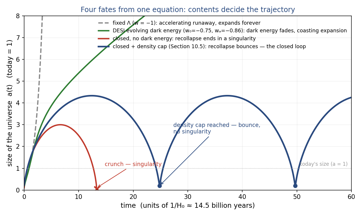
STATUS — Illustrative solutions of established equations. All four curves solve Eq. (12.12); the closed-loop curve additionally assumes the density cap, which is published but untested physics. No curve here is a prediction. The figure shows what is at stake in the sign and future of Q — the difference between runaway, crunch, and closed loop.

12.7 The Loop Without Time: A Phase Portrait, and the Sectors as Opposites

The trajectories of Figure 2 keep time on the horizontal axis, and with time as an axis a cyclic universe looks like history repeating from a start. But time is not a fundamental axis of the equations — it is a parameter along a solution. Plot the state of the universe against itself and time disappears from the picture entirely. This is a phase portrait, the standard tool for showing that a system cycles, and it is drawn in Figure 3(a): the size of the universe against its expansion rate. The runaway escapes to the right forever. The crunch trajectory begins and ends at a singularity. And the framework’s universe is a closed orbit — a literal closed loop, traversed clockwise, with no beginning, no end, and no point on it privileged as “the start.” An observer’s “age of the universe” is nothing but their phase along the orbit, measured from the most recent bounce. This is the precise, defensible sense in which the steady-state instinct survives the cautionary verdict of Section 10.9: what is steady is the loop as a geometric object, not the observations at any point on it. Epochs are entirely real — the density varies enormously around the orbit, so the CMB, nucleosynthesis, and galaxy evolution all still happen exactly as observed — but no absolute beginning is required, and none exists anywhere on the curve.

One might ask for size against energy density instead. In this model the density is fixed by the size alone, so expansion and contraction retrace a single curve — the picture closes into a loop only when the second coordinate distinguishes outbound from inbound, and that is what the expansion rate does. Density instead plays its role in panel (b), where the question “are virtual space and real space opposites?” receives a sharp, quantitative answer. The bounce correction of Eq. (12.13) can be rewritten, exactly, as a second energy component in the standard Friedmann equation:

H² = (8πG/3) · [ ρ + ρ_vir ] (12.14)

ρ_vir ≡ −ρ² / ρ_c (12.15)

ρ_vir — the virtual mirror term — an effective energy density with the opposite sign, negligible when space is dilute and dominant at maximum compression

Substituting Eq. (12.15) into Eq. (12.14) reproduces Eq. (12.13) identically — this is pure algebra, and it is exactly how the loop-quantum-cosmology effective equation is standardly written. Read through the framework, it says: the density cap behaves as a mirror sector whose contribution is opposite in sign to the real one, growing as the square of the real density. When compression reaches the cap, the two sectors meet as equal opposites, the effective total vanishes, the expansion rate passes through zero, and the collapse reverses. Figure 3(b) draws this across one cycle: the real density, its negative mirror image, and the effective total touching zero precisely at the bounce. The rewriting is not mine; the identification of ρ_vir with the virtual sector of Sections 3 and 4 — conversion running hard in reverse at maximum compression — is the framework’s conjecture, and I flag it as such.

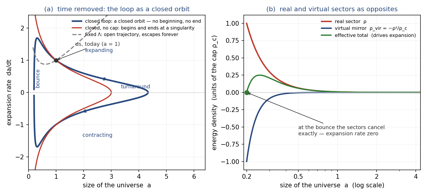
STATUS — A re-plotting and a reinterpretation. Panel (a) contains no new physics: it is the same solutions as Figure 2 with time removed as an axis, and it states the honest form of the steady-state claim — eternal loop, real epochs, no beginning. Eqs. (12.14)–(12.15) are algebraically identical to the published bounce correction; reading ρ_vir as the virtual sector is the conjecture. A genuine derivation would have to produce the −ρ²/ρ_c form from the conversion term Q of Eq. (12.4), which has not been done.

12.8 What This Calculation Establishes — and What It Does Not

Established by this section: the framework now has a dictionary from mechanism to observable (Q to w(z)); the global books close by construction, answering Section 8’s demand; the simplest conversion terms are solvable, and one is already disfavored by data — proof that the framework is falsifiable in practice, not just in principle; and the qualitative shape the data prefers (evolving w, phantom crossing, wₐ negative) is what an exchange naturally produces. Not established: the microphysics of Q. Nothing here derives the conversion rate from the structure of spacetime — Sections 3 and 10.2 owe that derivation, presumably through the thermodynamic-gravity route. Nor has this touched perturbations: interacting dark energy alters the growth of structure, and the growth data (Section 11, item 4) is a stringent test this background-level calculation has not yet faced. The DESI evidence itself remains contested (Section 10.8). But the framework has crossed the line I set in Section 9: it has produced numbers that can be wrong.

STATUS — A model now, not just a picture. One assumption (an exchange term), two exact solutions, one figure, one prediction. The next calculation is the perturbation analysis; the one after that is deriving Q from first principles.

13. The Seed: The Activation-Energy Notebook (2014)

The framework in this document did not begin with cosmology. It began in July 2014, in a lab notebook (Project 3, Book 778, copied from Book 777, dated 07/16/2014), with a chemistry analogy: treat conversion between the vacuum and the real state as a chemical reaction, with an activation energy, a reaction coordinate, and a spontaneity test. This section reproduces the notebook’s eleven plots, exactly as drawn, and translates its reasoning into the language the rest of the document now uses. The seed contains, in embryo, nearly every idea developed above: the conversion term Q of Section 12.2, the location-dependence of Section 3, the question of whether the exchange is bounded (Sections 10.5 and 12.6), and even the identification of converted vacuum with the dark sector (Sections 4 and 6). It also contains one conclusion the mature framework rejects, recorded honestly in 13.2.

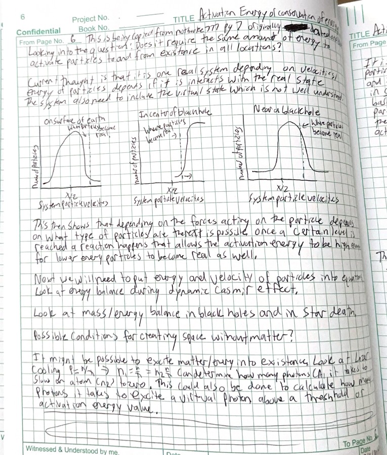
13.1 The Reaction Analogy: Conversion Has an Activation Barrier

In chemistry, a reaction converting reactants to products must pass over an energy barrier — the activation energy — whether the destination is lower in energy (exothermic, ΔH down) or higher (endothermic, ΔH up). Figure 4 reproduces the notebook’s two reference diagrams. The notebook’s move, prompted by the dynamic Casimir effect of Section 2.1, was to read vacuum-to-real conversion the same way: creating real photons from the vacuum is “endothermic” — energy must be supplied, by the fluctuating boundary in the laboratory — and returning photons to the vacuum is “exothermic.” Figure 5 reproduces the four conversion diagrams, drawn with respect to the real and virtual states. In the mature framework’s language, the barrier is why conversion does not simply happen everywhere at all times: Q in Eq. (12.4) is a rate, and rates are controlled by barriers. The rigorous counterpart of the intuition exists in the literature: transitions between vacuum states in quantum field theory (false-vacuum decay, Coleman 1977) are computed exactly as barrier-penetration problems — an activation picture, made precise.

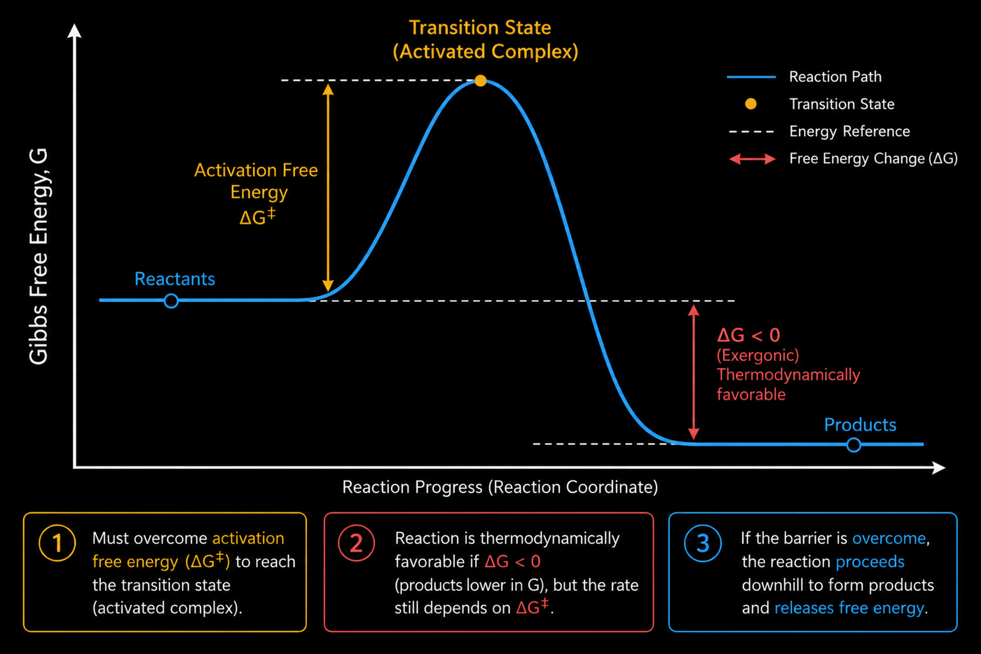
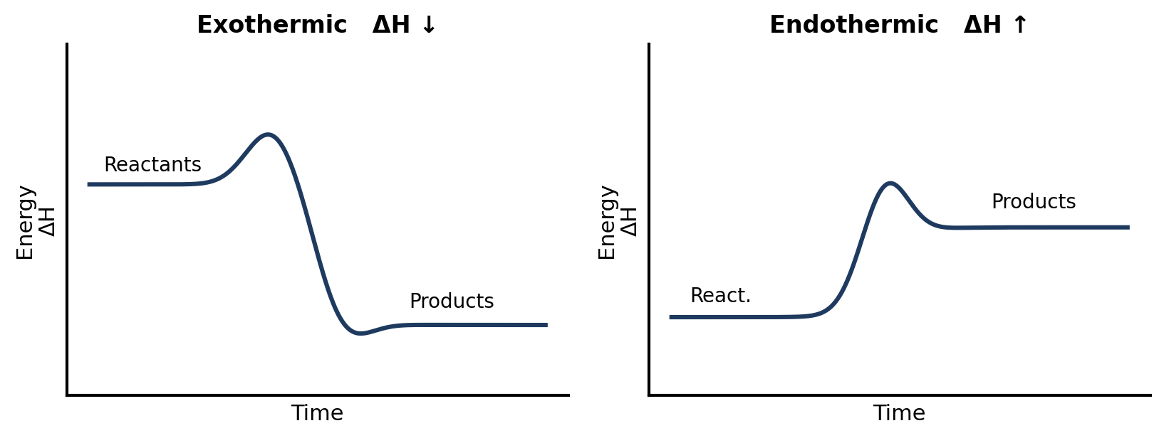
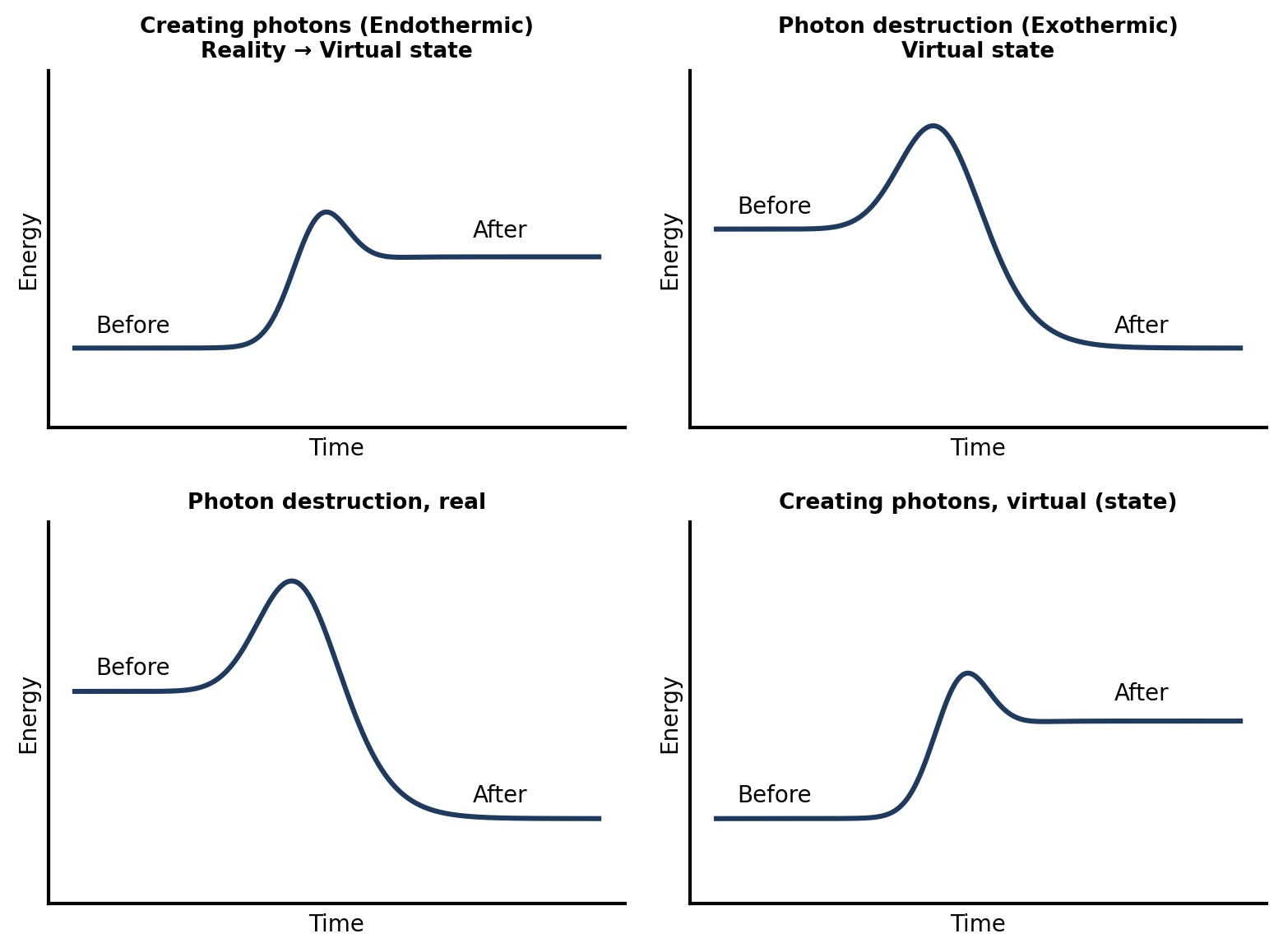
STATUS — Heuristic analogy, deliberately retained. Chemical kinetics does not literally govern the quantum vacuum. But barrier-controlled transition rates are exactly how physics treats decay between metastable states — false-vacuum decay is the published, quantitative version — so the analogy points at real machinery rather than away from it.

13.2 Spontaneity: The ΔG Test, and a Correction the Framework Made

The notebook then applied the chemist’s spontaneity criterion, ΔG = ΔH − TΔS: a process runs on its own when ΔG is negative. Creating photons from the vacuum has ΔH positive — energy is absorbed into the real state — so it can be spontaneous only if entropy rises enough, and the notebook noted that the entropy of the real state does increase when new particles appear. Where the energy cannot come from a heat bath, the process needs an activation source: the fluctuating mirror in the laboratory and, as the framework later proposed, the structure of spacetime in nature (Section 3). Read with Section 12 in hand, this is the embryonic conversion term: what the notebook called activation, the mature framework calls Q, and the notebook’s call to find “quantified values for S and H for virtual particles” is precisely the microphysics that Section 12.8 lists as still owed.

One correction, recorded plainly. The notebook entertained a sharper conclusion: that photon creation without an energy balance would show “energy of our universe can in fact increase,” breaking the first law — and that reverse conversion might break the second. The mature framework rejects that reading, and the difference is the whole point of Section 12.2: the books balance exactly, because what the real sector gains the vacuum sector loses. Conversion is an exchange, not creation. What the notebook was groping toward is real — the loosening of global energy bookkeeping in an expanding universe (Section 5) — but the framework resolves it with a ledger, not a violation. Likewise, the notebook’s thought that non-conservation might tame the infinite mass at black-hole centres has been replaced by the density cap of Sections 10.5 and 12.6–12.7, which needs no broken laws.

STATUS — Superseded in part, on purpose. The 2014 text reached for law-breaking where the 2026 framework reaches for two-sector bookkeeping. Recording the correction is part of the standard set in the preface: the framework’s history is evidence of how it responds to its own errors.

13.3 Location-Dependence: Where Particles Become Real

The notebook’s most distinctive idea is drawn in Figures 6 and 7. Treat the vacuum at a location as a population — a distribution over states, drawn in analogy to a Maxwell–Boltzmann velocity distribution — and mark a threshold: the level a fluctuation must reach to become real. On the surface of the Earth (Figure 6, left), the threshold sits far out in the tail: essentially nothing crosses, and the vacuum looks inert — consistent with the precision tests of Section 11, item 9. At the centre of a black hole (Figure 6, middle), the notebook drew the population piled up above the threshold: nearly everything crosses — the regime Section 3.1 flags as the framework’s open conjecture. Near a black hole (Figure 6, right), the threshold sits on the shoulder of the distribution: a meaningful fraction converts — the Hawking-radiation case of Section 3.1. Figure 7 then makes the deeper claim: the threshold itself may sit at different places in different locations. The same population appears with the line on the rising side (Location A — conversion is cheap) and on the descending side (Location B — conversion is dear). This is exactly the proposal the framework later formalized as “the structure of spacetime sets the local exchange rate” (Section 3), and the question the notebook wrote in 2014 — does activation cost the same everywhere? — is the one Section 3.2 holds as a conjecture and Section 11, item 8, subjects to the equivalence-principle bound.

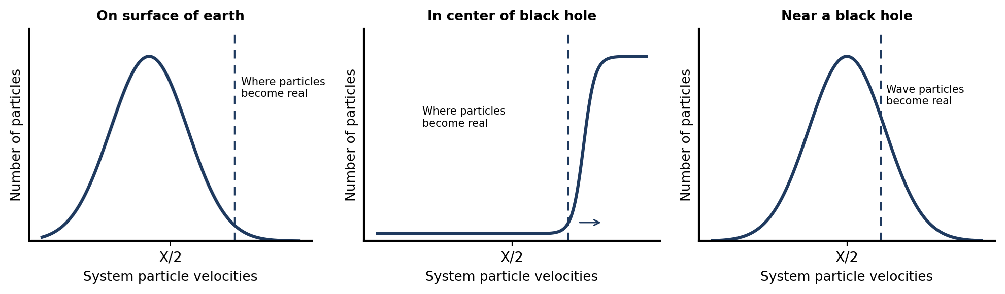
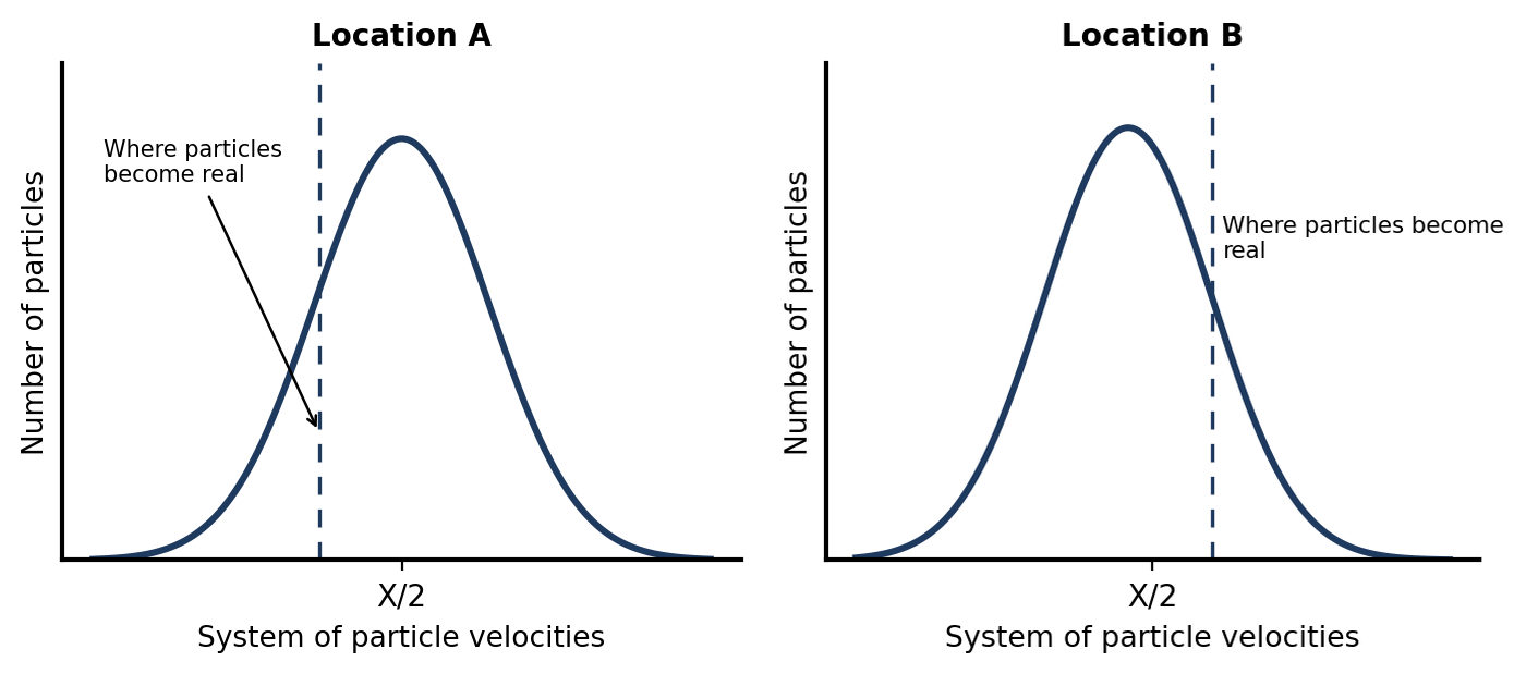
STATUS — The framework’s central conjecture, in its original form. These plots are qualitative by construction — the axes carry no units, and the notebook says so. Their content survives in Section 3 as the governing proposal, constrained by Section 11 items 8 and 9 to regimes the laboratory cannot reach.

13.4 The 2014 Questions, Answered by This Document

The notebook closed with three questions to investigate. Eleven years later, this document is the state of those investigations. First: “Is virtual matter or energy that is converted actually dark matter / energy?” For dark energy, the framework’s answer is a qualified yes — the vacuum sector in exchange, Sections 4 and 12, with the DESI inversion of Section 12.5 as its first quantitative contact. For dark matter, the framework remains silent and compatible (Section 6). Second: “Is there a limit to how much mass/energy can be brought into existence?” In the mature framework, yes: the density cap ρ_c of Sections 10.5 and 12.6–12.7, at which the real and virtual sectors cancel as equal opposites. Third: “Does it require the same amount of energy to activate particles to and from existence in all locations?” This remains the open conjecture of Section 3.2 — alive only in regimes the equivalence-principle and vacuum-precision tests of Section 11 cannot reach, which is exactly where the notebook’s black-hole plots placed it. The seed asked the right questions; the tree is the attempt to answer them without breaking anything that is measured.

STATUS — Provenance. Dated and preserved: notebook 777 page 5 onward, copied to Book 778, July 16, 2014. The plots in Figures 4–7 are the notebook’s final approved renderings, regenerated from the author’s own script (Appendix A.4).

References

The works named in this document, gathered in one place. The four foundational Einstein papers come first; the remainder are grouped by theme in roughly the order the document draws on them. The text refers to these works by author and year; the numbers are for navigation.

The Foundations: Einstein’s Papers

Relativistic Cosmology: The Equations and Their First Tests

The Quantum Vacuum (Sections 2, 11 item 9, 13)

Particle Production, Black Holes, and Their Observation (Sections 3, 7.3, 10.7, 11 items 7–8)

Horizon Thermodynamics and Emergent Gravity (Sections 10.1–10.2)

Cosmologies Without an Initial Singularity (Sections 1, 7, 10.3–10.5, 10.9, 12.6–12.7)

Rotation, Orbits, and the Shape of the Universe (Sections 7.2–7.3)

Observational Cosmology and the Dark Sector (Sections 4–6, 10.6, 10.8, 11, 12.5)

Interacting Dark Energy (Sections 12.2–12.5)

Primary Source

Appendix A — Plot Generation Source Code

The scripts below are the complete, self-contained sources used to generate Figures 1, 2, and 3, plus the assembly step for the notebook plates of Figures 4–7. All are written in Python 3 and require the NumPy and Matplotlib libraries; Figure 2 additionally requires SciPy, and A.4 requires Pillow. Running any file as-is reproduces its figure exactly.

A.1 — Source for Figure 1 (effective w(z) against DESI DR2)

This script computes the exact solution of Worked Example B (Eqs. 12.9–12.10), forms the effective equation of state as an observer would (Section 12.4), overlays the DESI DR2 central curves, and marks the sign flip of Q implied by Eq. (12.11). The closed-form solutions it uses were independently verified by direct numerical integration of Eqs. (12.4)–(12.5).

# Figure 1 — Effective dark-energy behaviour of the conversion term Q,
# against the DESI DR2 central values.
# Requires: Python 3, NumPy, Matplotlib.  Run:  python3 plot_figure1.py
 
import numpy as np
import matplotlib
matplotlib.use('Agg')
import matplotlib.pyplot as plt
 
# ---- Cosmological parameters and Worked Example B (Section 12.4) ----
Om, Ov, alpha = 0.31, 0.69, 0.03        # matter, vacuum densities; coupling
 
def rho_de_fit(a):
    """Effective dark-energy density seen by an observer who assumes
    matter dilutes exactly as a^-3 (Eqs. 12.9-12.10 minus Om*a^-3)."""
    return (Ov + (alpha/(1-alpha))*Om*(a**(-3*(1-alpha)) - 1)
            + Om*(a**(-3*(1-alpha)) - a**(-3)))
 
def w_eff(a):
    """Effective equation of state: 1+w = -(1/3) d ln(rho_de)/d ln(a)."""
    d = 3*Om*(a**(-3) - a**(-3*(1-alpha)))   # d rho_de_fit / d ln a
    return -(1/3)*d/rho_de_fit(a) - 1
 
# ---- Curves ----
z = np.linspace(0, 1.4, 400)
a = 1/(1+z)
wB    = np.array([w_eff(x) for x in a])            # Example B
wDESY = -0.750 - 0.86*z/(1+z)                      # DESI DR2+CMB+DESY5 (CPL)
wPP   = -0.838 - 0.62*z/(1+z)                      # DESI DR2+CMB+Pantheon+
 
# ---- Plot ----
BLUE, GRAY, ORANGE, GREEN = '#2A4A7F', '#888888', '#C0392B', '#2E7D32'
fig, ax = plt.subplots(figsize=(8.2, 4.9), dpi=150)
 
ax.axhline(-1, color=GRAY, lw=1.2, ls='--')
ax.text(1.32, -0.985, 'LCDM  (w = -1)', color=GRAY, fontsize=9, ha='right')
 
ax.axhline(-0.9, color=GREEN, lw=2)                # Example A (Section 12.3)
ax.text(1.32, -0.885, 'Example A:  Q = 3aH rho_v,  a = 0.1  (constant w)',
        color=GREEN, fontsize=9, ha='right')
 
ax.plot(z, wB, color=BLUE, lw=2.5,
        label='Example B:  Q = 3aH rho_m,  a = 0.03  (phantom crossing)')
ax.plot(z, wDESY, color=ORANGE, lw=2.2,
        label='DESI DR2 + CMB + DESY5  (w0 = -0.75, wa = -0.86)')
ax.plot(z, wPP, color=ORANGE, lw=1.6, ls=':',
        label='DESI DR2 + CMB + Pantheon+  (w0 = -0.838, wa = -0.62)')
 
# ---- Mark the sign flip of Q implied by the DESI curve (Eq. 12.11) ----
zstar = 0.41                                        # -(1+w0)/wa -> z*
wstar = -0.750 - 0.86*zstar/(1+zstar)
ax.plot([zstar], [wstar], 'o', color=ORANGE, ms=7)
ax.annotate('conversion direction flips\n(Q = 0 at z ~ 0.4)',
            xy=(zstar, wstar), xytext=(0.62, -0.83), fontsize=9,
            color=ORANGE, arrowprops=dict(arrowstyle='->', color=ORANGE))
ax.text(0.02, -0.79, 'Q > 0 :  vacuum -> real sector', fontsize=9)
ax.text(0.80, -1.32, 'Q < 0 :  real sector -> vacuum', fontsize=9)
 
ax.set_xlim(0, 1.4); ax.set_ylim(-1.55, -0.72)
ax.set_xlabel('redshift  z'); ax.set_ylabel('effective equation of state  w(z)')
ax.set_title('Effective dark-energy behaviour of the conversion term Q,'
             ' against DESI DR2', fontsize=11.5, color='#2A4A7F')
ax.legend(loc='lower left', fontsize=8.6, frameon=False)
ax.grid(alpha=0.25, lw=0.6)
plt.tight_layout()
plt.savefig('fig_weff.png', dpi=150)

A.2 — Source for Figure 2 (four fates of the universe)

This script integrates Eq. (12.12) as a second-order equation for a(t), which lets the solver pass smoothly through turnarounds where the expansion halts and reverses. The four trajectories differ only in the contents supplied to the same equation; the closed-loop curve applies the density-cap correction of Eq. (12.13).

# Figure 2 — Four fates of the universe from the same Friedmann equation
# (Eq. 12.12), differing only in contents.  Requires: NumPy, SciPy, Matplotlib.
 
import numpy as np
from scipy.integrate import solve_ivp
import matplotlib
matplotlib.use('Agg')
import matplotlib.pyplot as plt
 
# (da/dt)^2 = E(a) in units where H0 = 1.  Integrating the equivalent
# second-order form  d2a/dt2 = E'(a)/2  handles turnarounds automatically.
def trajectory(E, a0, t_max, adot0=None, eps=1e-5):
    dE = lambda a: (E(a+eps) - E(a-eps)) / (2*eps)
    if adot0 is None:
        adot0 = np.sqrt(max(E(a0), 0.0))
    hit_zero = lambda t, y: y[0] - 0.02          # stop if a -> 0 (crunch)
    hit_zero.terminal, hit_zero.direction = True, -1
    hit_top = lambda t, y: y[0] - 9.5            # stop once off the top of the plot
    hit_top.terminal, hit_top.direction = True, 1
    sol = solve_ivp(lambda t, y: [y[1], 0.5*dE(y[0])], [0, t_max],
                    [a0, adot0], events=[hit_zero, hit_top], max_step=0.1,
                    rtol=1e-8, atol=1e-10)
    return sol.t, sol.y[0]
 
# ---- Contents of the four universes (today's units: critical density = 1) ----
w0, wa = -0.75, -0.86                             # DESI DR2 central values
f_cpl = lambda a: a**(-3*(1+w0+wa)) * np.exp(-3*wa*(1-a))
 
E_lcdm = lambda a: 0.31/a + 0.69*a**2             # fixed cosmological constant
E_cpl  = lambda a: 0.31/a + 0.69*f_cpl(a)*a**2    # DESI evolving dark energy
E_closed = lambda a: 1.50/a - 0.50                # closed, no dark energy
rho_c = 1.30/0.20**3                              # density cap -> bounce at a~0.2
E_loop = lambda a: (1.30/a - 0.30)*(1 - (1.30/a**3)/rho_c)   # Eq. (12.13)
 
t1, a1 = trajectory(E_lcdm,  0.10, 60)
t2, a2 = trajectory(E_cpl,   0.10, 60)
t3, a3 = trajectory(E_closed, 0.10, 60)
t4, a4 = trajectory(E_loop,  0.21, 60)
 
# ---- Plot ----
BLUE, GRAY, ORANGE, GREEN = '#2A4A7F', '#888888', '#C0392B', '#2E7D32'
fig, ax = plt.subplots(figsize=(8.2, 4.9), dpi=150)
ax.plot(t1, a1, color=GRAY,  ls='--', lw=2,  label='fixed Λ (w = −1): accelerating runaway, expands forever')
ax.plot(t2, a2, color=GREEN, lw=2.2, label='DESI evolving dark energy (w₀=−0.75, wₐ=−0.86): dark energy fades, coasting expansion')
ax.plot(t3, a3, color=ORANGE, lw=2.2, label='closed, no dark energy: recollapse ends in a singularity')
ax.plot([t3[-1]], [0.05], 'x', color=ORANGE, ms=9, mew=2.5)
ax.annotate('crunch — singularity', xy=(t3[-1], 0.1), xytext=(t3[-1]+1.5, 1.1),
            fontsize=9, color=ORANGE, arrowprops=dict(arrowstyle='->', color=ORANGE))
ax.plot(t4, a4, color=BLUE,  lw=2.6, label='closed + density cap (Section 10.5): recollapse bounces — the closed loop')
 
# annotate bounces on the closed-loop curve
mins = (np.r_[False, (a4[1:-1] < a4[:-2]) & (a4[1:-1] < a4[2:]), False])
for tb, ab in zip(t4[mins], a4[mins]):
    ax.plot([tb], [ab], 'o', color=BLUE, ms=6)
if mins.any():
    tb, ab = t4[mins][0], a4[mins][0]
    ax.annotate('density cap reached — bounce,\nno singularity', xy=(tb, ab),
                xytext=(tb+2.5, 2.6), fontsize=9, color=BLUE,
                arrowprops=dict(arrowstyle='->', color=BLUE))
 
ax.axhline(1, color='#BBBBBB', lw=0.8, ls=':')
ax.text(59.3, 1.12, "today's size (a = 1)", color='#999999', fontsize=8, ha='right')
ax.set_xlim(0, 60); ax.set_ylim(0, 8)
ax.set_xlabel('time  (units of 1/H₀ ≈ 14.5 billion years)', fontsize=11)
ax.set_ylabel('size of the universe  a(t)   (today = 1)', fontsize=11)
ax.set_title('Four fates from one equation: contents decide the trajectory', fontsize=11.5, color='#2A4A7F')
ax.legend(loc='upper right', fontsize=8.4, frameon=False)
ax.grid(alpha=0.25, lw=0.6)
plt.tight_layout()
plt.savefig('fig_fates.png', dpi=150)
print('bounce times:', np.round(t4[mins], 1))

A.3 — Source for Figure 3 (the loop without time; sectors as opposites)

This script draws the phase portrait of Eq. (12.12) — size against expansion rate, on which the cyclic solution is a closed orbit — and the sector decomposition of Eqs. (12.14)–(12.15), in which the real density and the virtual mirror term cancel exactly at the bounce. No differential equation needs solving here: the phase-space curves follow directly from the energy relation (da/dt)² = E(a).

# Figure 3 — The closed loop without time.
# (a) Phase portrait: size vs expansion rate; a cycle is a closed orbit.
# (b) Size vs energy density: real sector and virtual mirror as opposites.
# Requires: NumPy, Matplotlib.  Units: H0 = 1; densities in units of the cap.
 
import numpy as np
import matplotlib
matplotlib.use('Agg')
import matplotlib.pyplot as plt
 
rho_c  = 1.30/0.20**3                              # density cap -> bounce at a = 0.2
V_loop = lambda a: (1.30/a - 0.30)*(1 - (1.30/a**3)/rho_c)   # closed loop (Eq. 12.13)
V_crun = lambda a: 1.50/a - 0.50                             # closed, no cap
V_lcdm = lambda a: 0.31/a + 0.69*a**2                        # fixed cosmological constant
 
BLUE, GRAY, ORANGE, GREEN = '#2A4A7F', '#888888', '#C0392B', '#2E7D32'
fig, (ax1, ax2) = plt.subplots(1, 2, figsize=(9.6, 4.4), dpi=150)
 
# ---------------- panel (a): phase portrait ----------------
a_min, a_max = 0.20, 13/3                          # V_loop = 0 exactly here
al = np.linspace(a_min*1.0005, a_max*0.9995, 800)
vl = np.sqrt(np.clip(V_loop(al), 0, None))
ax1.plot(np.r_[al, al[::-1]], np.r_[vl, -vl[::-1]], color=BLUE, lw=2.6,
         label='closed loop: a closed orbit — no beginning, no end')
 
ac = np.linspace(0.16, 3*0.9995, 600)              # crunch universe, turnaround a = 3
vc = np.sqrt(np.clip(V_crun(ac), 0, None))
ax1.plot(np.r_[ac, ac[::-1]], np.r_[vc, -vc[::-1]], color=ORANGE, lw=1.8,
         label='closed, no cap: begins and ends at a singularity')
ax1.plot([ac[0], ac[0]], [vc[0], -vc[0]], 'x', color=ORANGE, ms=9, mew=2.5)
 
aL = np.linspace(0.16, 9, 400)
ax1.plot(aL, np.sqrt(V_lcdm(aL)), color=GRAY, ls='--', lw=1.8,
         label='fixed Λ: open trajectory, escapes forever')
ax1.plot([1], [1], 'o', color='#333333', ms=6)
ax1.annotate('us, today (a = 1)', xy=(1, 1), xytext=(1.7, 1.45),
             fontsize=8.5, color='#333333',
             arrowprops=dict(arrowstyle='->', color='#333333', lw=0.9))
 
# circulation arrows on the loop (clockwise)
for a_pt, sgn, dx in [(2.4, 1, .5), (2.4, -1, -.5)]:
    v_pt = sgn*np.sqrt(V_loop(a_pt))
    ax1.annotate('', xy=(a_pt+dx, sgn*np.sqrt(V_loop(a_pt+dx))),
                 xytext=(a_pt, v_pt),
                 arrowprops=dict(arrowstyle='-|>', color=BLUE, lw=1.6))
ax1.text(0.24, 0.18, 'bounce', fontsize=8.5, color=BLUE, rotation=90)
ax1.text(3.35, 0.13, 'turnaround', fontsize=8.5, color=BLUE)
ax1.text(2.05, 1.25, 'expanding', fontsize=8.5, color=BLUE)
ax1.text(1.95, -1.38, 'contracting', fontsize=8.5, color=BLUE)
ax1.axhline(0, color='#CCCCCC', lw=0.7)
ax1.set_xlim(0, 6.4); ax1.set_ylim(-2.4, 2.4)
ax1.set_xlabel('size of the universe  a'); ax1.set_ylabel('expansion rate  da/dt')
ax1.set_title('(a)  time removed: the loop as a closed orbit', fontsize=10.5, color=BLUE)
ax1.legend(loc='upper right', fontsize=7.4, frameon=False)
ax1.grid(alpha=0.22, lw=0.5)
 
# ---------------- panel (b): real vs virtual sectors ----------------
ab = np.geomspace(a_min, a_max, 500)
r_real = (1.30/ab**3)/rho_c                        # real density, units of the cap
r_vir  = -r_real**2                                # mirror term (Eq. 12.15)
r_eff  = r_real + r_vir
 
ax2.plot(ab, r_real, color=ORANGE, lw=2.2, label='real sector  ρ')
ax2.plot(ab, r_vir,  color=BLUE,   lw=2.2, label='virtual mirror  ρ_vir = −ρ²/ρ_c')
ax2.plot(ab, r_eff,  color=GREEN,  lw=2.0, label='effective total  (drives expansion)')
ax2.axhline(0, color='#CCCCCC', lw=0.8)
ax2.plot([a_min], [0], 'o', color=GREEN, ms=7)
ax2.annotate('at the bounce the sectors cancel\nexactly — expansion rate zero',
             xy=(a_min, 0), xytext=(0.5, -0.62), fontsize=8.5, color='#333333',
             arrowprops=dict(arrowstyle='->', color='#333333', lw=0.9))
ax2.set_xscale('log')
ax2.set_xlim(a_min*0.95, a_max); ax2.set_ylim(-1.12, 1.12)
ax2.set_xticks([0.2, 0.5, 1, 2, 4]); ax2.set_xticklabels(['0.2','0.5','1','2','4'])
ax2.set_xlabel('size of the universe  a  (log scale)')
ax2.set_ylabel('energy density  (units of the cap ρ_c)')
ax2.set_title('(b)  real and virtual sectors as opposites', fontsize=10.5, color=BLUE)
ax2.legend(loc='upper right', fontsize=7.8, frameon=False)
ax2.grid(alpha=0.22, lw=0.5)
 
plt.tight_layout()
plt.savefig('fig_loop.png', dpi=150)
print('saved')

A.4 — Assembly of Figures 4–7 (the notebook plates)

The eleven underlying plots of Figures 4–7 are generated by the author’s own script, activation_energy_plots.py (2014 notebook, final approved renderings; distributed alongside this document rather than reproduced here, at roughly 250 lines). The short script below then assembles them into the four plates: Figure 4 pairs the reaction-coordinate templates, Figure 5 grids the four photon-conversion diagrams, Figure 6 rows the three location plots, and Figure 7 pairs Locations A and B.

# Composites for Figures 4-7 from the notebook generator's output (./graphs/).
# Run activation_energy_plots.py first, then this file.  Requires: Pillow.
 
from PIL import Image
 
def row(files):
    ims = [Image.open(f) for f in files]
    h = max(i.height for i in ims); W = sum(i.width for i in ims)
    out = Image.new('RGB', (W, h), 'white'); x = 0
    for i in ims:
        out.paste(i, (x, (h - i.height)//2)); x += i.width
    return out
 
def grid2x2(files):
    a, b, c, d = [Image.open(f) for f in files]
    W = a.width + b.width; H = a.height + c.height
    out = Image.new('RGB', (W, H), 'white')
    out.paste(a, (0, 0));        out.paste(b, (a.width, 0))
    out.paste(c, (0, a.height)); out.paste(d, (a.width, a.height))
    return out
 
g = lambda i: f'graphs/image{i}.png'
row([g(1), g(2)]).save('fig4_notebook_reactions.png')          # Figure 4
grid2x2([g(3), g(4), g(5), g(6)]).save('fig5_notebook_photons.png')  # Figure 5
row([g(7), g(8), g(9)]).save('fig6_notebook_locations.png')    # Figure 6
row([g(10), g(11)]).save('fig7_notebook_AB.png')               # Figure 7
print('composites written')